This notebook replicates the models in chapter 12 of Godley and Lavoie (2007).
library(sfcr)
library(tidyverse)
#> ── Attaching packages ─────────────────────────────────────── tidyverse 1.3.1 ──
#> ✔ ggplot2 3.3.5     ✔ purrr   0.3.4
#> ✔ tibble  3.1.5     ✔ dplyr   1.0.7
#> ✔ tidyr   1.1.4     ✔ stringr 1.4.0
#> ✔ readr   2.0.2     ✔ forcats 0.5.1
#> ── Conflicts ────────────────────────────────────────── tidyverse_conflicts() ──
#> ✖ dplyr::filter() masks stats::filter()
#> ✖ dplyr::lag()    masks stats::lag()
Model skeleton
open12_ext <- sfcr_set(
  alpha1_uk ~ 0.75,
  alpha1_us ~ 0.75,
  alpha2_uk ~ 0.13333,
  alpha2_us ~ 0.13333,
  eps0 ~ - 2.1,
  eps1 ~ 0.7,
  eps2 ~ 1,
  lambda10 ~ 0.7,
  lambda11 ~ 5,
  lambda12 ~ 5,
  lambda20 ~ 0.25,
  lambda21 ~ 5,
  lambda22 ~ 5,
  lambda40 ~ 0.7,
  lambda41 ~ 5,
  lambda42 ~ 5,
  lambda50 ~ 0.25,
  lambda51 ~ 5,
  lambda52 ~ 5,
  mu0 ~ - 2.1,
  mu1 ~ 0.7,
  mu2 ~ 1,
  nu0m ~ - 0.00001,
  nu0x ~ - 0.00001,
  nu1m ~ 0.7,
  nu1x ~ 0.5,
  phi_uk ~ 0.2381,
  phi_us ~ 0.2381,
  theta_uk ~ 0.2,
  theta_us ~ 0.2,


  # Exogenous variables
  #b_cb_ukus_s ~ 0.02031,
  dxre_us ~ 0,
  g_k_uk ~ 16,
  g_k_us ~ 16,
  or_uk ~ 7,
  pg_us ~ 1,
  pr_uk ~ 1.3333,
  pr_us ~ 1.3333,
  #r_uk ~ 0.03,
  r_us ~ 0.03,
  w_uk ~ 1,
  w_us ~ 1,

  #xr_uk ~ 1.0003,
  #xr_us ~ 0.99971,
  xre_uk ~ 1.0003,
  xre_us ~ 0.99971,
  or_us ~ 7,
  dxre_uk ~ 0,


)


open12_init <- sfcr_set(

  # Exogenous

  b_cb_ukus_s ~ 0.02031,
  dxre_us ~ 0,
  g_k_uk ~ 16,
  g_k_us ~ 16,
  or_uk ~ 7,
  pg_us ~ 1,
  pr_uk ~ 1.3333,
  pr_us ~ 1.3333,
  r_uk ~ 0.03,
  r_us ~ 0.03,
  w_uk ~ 1,
  w_us ~ 1,

  # Endogenous

  b_cb_ukuk_d ~ 0.27984,
  b_cb_ukuk_s ~ 0.27984,
  b_cb_ukuk_sa ~ 0.27984,
  b_cb_ukus_d ~ 0.0203,
  b_cb_usus_d ~ 0.29843,
  b_cb_usus_s ~ 0.29843,
  b_uk_s ~ 138.94,
  b_ukuk_d ~ 102.18,
  b_ukuk_s ~ 102.18,
  b_ukus_d ~ 36.493,
  b_ukus_s ~ 36.504,
  b_us_s ~ 139.02,
  b_usuk_d ~ 36.497,
  b_usuk_s ~ 36.487,
  b_usus_d ~ 102.19,
  b_usus_s ~ 102.19,
  h_uk_d ~ 7.2987,
  h_uk_s ~ 7.2987,
  h_us_d ~ 7.2995,
  h_us_s ~ 7.2995,
  or_us ~ 7,
  v_k_uk ~ 152.62,
  v_k_us ~ 152.63,
  v_uk ~ 145.97,
  v_us ~ 145.99001,

  # Other endogenous
  c_k_uk ~ 81.393,
  c_k_us ~ 81.401,
  cab_uk ~ 0,
  cab_us ~ 0,
  cons_uk ~ 77.851,
  cons_us ~ 77.86,
  ds_k_uk ~ 97.393,
  ds_k_us ~ 97.401,
  ds_uk ~ 93.154,
  ds_us ~ 93.164,
  dxre_uk ~ 0,
  f_cb_uk ~ 0.00869,
  f_cb_us ~ 0.00895,
  g_uk ~ 15.304,
  g_us ~ 15.304,
  im_k_uk ~ 11.928,
  im_k_us ~ 11.926,
  im_uk ~ 11.407,
  im_us ~ 11.409,
  kabp_uk ~ 0.00002,
  kabp_us ~ - 0.00002,
  n_uk ~ 73.046,
  n_us ~ 73.054,
  pds_uk ~ 0.95648,
  pds_us ~ 0.95649,
  pg_uk ~ 0.99971,
  pm_uk ~ 0.95628,
  pm_us ~ 0.95661,
  ps_uk ~ 0.95646,
  ps_us ~ 0.9565,
  px_uk ~ 0.95634,
  px_us ~ 0.95656,
  py_uk ~ 0.95648,
  py_us ~ 0.95649,
  s_k_uk ~ 109.32,
  s_k_us ~ 109.33,
  s_uk ~ 104.56,
  s_us ~ 104.57,
  t_uk ~ 19.463,
  t_us ~ 19.465,
  x_k_uk ~ 11.926,
  x_k_us ~ 11.928,
  x_uk ~ 11.406,
  x_us ~ 11.41,
  xr_uk ~ 1.0003,
  xr_us ~ 0.99971,
  xre_uk ~ 1.0003,
  xre_us ~ 0.99971,
  y_k_uk ~ 97.392,
  y_k_us ~ 97.403,
  y_uk ~ 93.154,
  y_us ~ 93.164,
  yd_uk ~ 77.851,
  yd_us ~ 77.86,
  ydhs_k_uk ~ 81.394,
  ydhs_k_us ~ 81.402,
  ydhse_k_uk ~ 81.394,
  ydhse_k_us ~ 81.402
)
open12_eqs <- sfcr_set(

# Disposable income in UK - eq. 12.1
yd_uk ~ (y_uk + r_uk[-1]*b_ukuk_d[-1] + xr_us*r_us[-1]*b_ukus_s[-1])*(1 - theta_uk) + (xr_us - xr_us[-1])*b_ukus_s[-1],

# Haig-Simons disposable income in UK - eq. 12.2
yd_hs_uk ~ yd_uk + (xr_us - xr_us[-1])*b_ukus_s[-1],

# Wealth accumulation in UK - eq. 12.3
v_uk ~ v_uk[-1] + yd_uk - cons_uk,

# Disposable income in US - eq. 12.4
yd_us ~ (y_us + r_us[-1]*b_usus_d[-1] + xr_uk*r_uk[-1]*b_usuk_s[-1])*(1 - theta_us) + (xr_uk - xr_uk[-1])*b_usuk_s[-1],


# Haig-Simons disposable income in US - eq. 12.5
yd_hs_us ~ yd_us + d(xr_uk)*b_usuk_s[-1],

# Wealth accumulation in US - eq. 12.6
v_us ~ v_us[-1] + yd_us - cons_us,

# Taxes in UK - eq. 12.7
t_uk ~ theta_uk*(y_uk + r_uk[-1]*b_ukuk_d[-1] + xr_us*r_us[-1]*b_ukus_s[-1]),

# Taxes in US - eq. 12.8
t_us ~ theta_us*(y_us + r_us[-1]*b_usus_d[-1] + xr_uk*r_uk[-1]*b_usuk_s[-1]),

# Equations 12.9 & 12.10 are dropped in favour of equations 12.53 & 12.54

# Profits of Central Bank in UK - eq. 12.11 - typo in the book for r_us
f_cb_uk ~ r_uk[-1]*b_cb_ukuk_d[-1] + r_us[-1]*b_cb_ukus_s[-1]*xr_us,

# Profits of Central Bank in US - eq. 12.12
f_cb_us ~ r_us[-1]*b_cb_usus_d[-1],

# Government budget constraint - UK - eq. 12.13
b_uk_s ~ b_uk_s[-1] + g_uk + r_uk[-1]*b_uk_s[-1] - t_uk - f_cb_uk,

# Government budget constraint - US - eq. 12.14
b_us_s ~ b_us_s[-1] + g_us + r_us[-1]*b_us_s[-1] - t_us - f_cb_us,

# Current account balance - UK - eq. 12.15
cab_uk ~ x_uk - im_uk + xr_us*r_us[-1]*b_ukus_s[-1] - r_uk[-1]*b_usuk_s[-1] + r_us[-1]*b_cb_ukus_s[-1]*xr_us,

# Capital account balance in UK - eq. 12.16
kab_uk ~ kabp_uk - (xr_us*(b_cb_ukus_s - b_cb_ukus_s[-1]) + pg_uk*(or_uk - or_uk[-1])),

# Current account balance in US - eq. 12.17
cab_us ~ x_us - im_us + xr_uk*r_uk[-1]*b_usuk_s[-1] - r_us[-1]*b_ukus_s[-1] - r_us[-1]*b_cb_ukus_s[-1],

# Capital account balance in US - eq. 12.18
kab_us ~ kabp_us + (b_cb_ukus_s - b_cb_ukus_s[-1]) - pg_us*(or_us - or_us[-1]),

# Capital account balance in UK, net of official transactions - eq. 12.19
kabp_uk ~ - (b_ukus_s - b_ukus_s[-1])*xr_us + (b_usuk_s - b_usuk_s[-1]),

# Capital account balance in US, net of official transactions - eq. 12.20
kabp_us ~ - (b_usuk_s - b_usuk_s[-1])*xr_uk + (b_ukus_s - b_ukus_s[-1]),


# TRADE

# Import prices in UK - eq. 12.21
pm_uk ~ exp(nu0m + nu1m*log(py_us) + (1 - nu1m)*log(py_uk) - nu1m*log(xr_uk)),

# Export prices in UK - eq. 12.22
px_uk ~ exp(nu0x + nu1x*log(py_us) + (1 - nu1x)*log(py_uk) - nu1x*log(xr_uk)),

# Export prices in US - eq. 12.23
px_us ~ pm_uk*xr_uk,

# Import prices in US - eq. 12.24
pm_us ~ px_uk*xr_uk,

# Real exports from UK - eq. 12.25 - depends on current relative price
x_k_uk ~ exp(eps0 - eps1*log(pm_us/py_us) + eps2*log(y_k_us)),

# Real imports of UK - eq. 12.26
im_k_uk ~ exp(mu0 - mu1*log(pm_uk[-1]/py_uk[-1]) + mu2*log(y_k_uk)),

# Real exports from US - eq. 12.27
x_k_us ~ im_k_uk,

# Real imports of US - eq. 12.28
im_k_us ~ x_k_uk,

# Exports of UK - eq. 12.29
x_uk ~ x_k_uk*px_uk,

# Exports of US - eq. 12.30
x_us ~ x_k_us*px_us,

# Imports of UK - eq. 12.31
im_uk ~ im_k_uk*pm_uk,

# Imports of US - eq. 12.32
im_us ~ im_k_us*pm_us,


# INCOME AND EXPENDITURE

# Real wealth in UK - eq. 12.33
v_k_uk ~ v_uk/pds_uk,

# Real wealth in US - eq. 12.34
v_k_us ~ v_us/pds_us,


# Real Haig-Simons disposable income in UK - eq. 12.35
ydhs_k_uk ~ yd_uk/pds_uk - v_k_uk[-1]*(pds_uk - pds_uk[-1])/pds_uk,

# Real Haig-Simons disposable income in US - eq. 12.36
ydhs_k_us ~ yd_us/pds_us - v_k_us[-1]*(pds_us - pds_us[-1])/pds_us ,

# Real consumption in UK - eq. 12.37
c_k_uk ~ alpha1_uk*ydhse_k_uk + alpha2_uk*v_k_uk[-1],

# Real consumption in US - eq. 12.38
c_k_us ~ alpha1_us*ydhse_k_us + alpha2_us*v_k_us[-1],

# Expected real Haig-Simons disposable income in UK - eq. 12.39
ydhse_k_uk ~ (ydhs_k_uk + ydhs_k_uk[-1])/2,

# Expected real Haig-Simons disposable income in US - eq. 12.40
ydhse_k_us ~ (ydhs_k_us + ydhs_k_us[-1])/2,

# Real sales in UK - eq. 12.41
s_k_uk ~ c_k_uk + g_k_uk + x_k_uk,

# Real sales in US - eq. 12.42
s_k_us ~ c_k_us + g_k_us + x_k_us,

# Value of sales in UK - eq. 12.43
s_uk ~ s_k_uk*ps_uk,

# Value of sales in US - eq. 12.44
s_us ~ s_k_us*ps_us,

# Price of sales in UK - eq. 12.45
ps_uk ~ (1 + phi_uk)*(w_uk*n_uk + im_uk)/s_k_uk,

# Price of sales in US - eq. 12.46
ps_us ~ (1 + phi_us)*(w_us*n_us + im_us)/s_k_us,

# Price of domestic sales in UK - eq. 12.47
pds_uk ~ (s_uk - x_uk)/(s_k_uk - x_k_uk),

# Price of domestic sales in US - eq. 12.48
pds_us ~ (s_us - x_us)/(s_k_us - x_k_us),

# Domestic sales in UK - eq. 12.49
ds_uk ~ s_uk - x_uk,

# Domestic sales in US - eq. 12.50
ds_us ~ s_us - x_us,

# Real domestic sales in UK - eq. 12.51
ds_k_uk ~ c_k_uk + g_k_uk,

# Real domestic sales in US - eq. 12.52
ds_k_us ~ c_k_us + g_k_us,

# Value of output in UK - eq. 12.53
y_uk ~ s_uk - im_uk,

# Value of output in US - eq. 12.54
y_us ~ s_us - im_us,

# Value of real output in UK - eq. 12.55
y_k_uk ~ s_k_uk - im_k_uk,

# Value of real output in US - eq. 12.56
y_k_us ~ s_k_us - im_k_us,

# Price of output in UK - eq. 12.57
py_uk ~ y_uk/y_k_uk,

# Price of output in US - eq. 12.58
py_us ~ y_us/y_k_us,

# Consumption in UK - eq. 12.59
cons_uk ~ c_k_uk*pds_uk,

# Consumption in US - eq. 12.60
cons_us ~ c_k_us*pds_us,

# Government expenditure in UK - eq. 12.61
g_uk ~ g_k_uk*pds_uk,

# Government expenditure in US - eq. 12.62
g_us ~ g_k_us*pds_us,

# Note: tax definitions in the book as eqns 12.63 & 12.64 are already as eqns 12.7 & 12.8

# Employment in UK - eq. 12.65
n_uk ~ y_k_uk/pr_uk,

# Employment in US - eq. 12.66
n_us ~ y_k_us/pr_us,

# ASSET DEMANDS

# Demand for UK bills in UK - eq. 12.67
b_ukuk_d ~ v_uk*(lambda10 + lambda11*r_uk - lambda12*(r_us + dxre_us)),

# Demand for US bills in UK - 12.68F
b_ukus_d ~ v_uk*(lambda20 - lambda21*r_uk + lambda22*(r_us + dxre_us)),

# Base interest rates r_uk - eq. 12.68R
# r_uk ~ (lambda20 + lambda22*(r_us + dxre_us) - b_ukus_d/v_uk)/lambda21,

# Demand for money in UK - eq. 12.69
h_uk_d ~ v_uk - b_ukuk_d - b_ukus_d,

# Demand for US bills in US - eq. 12.70
b_usus_d ~ v_us*(lambda40 + lambda41*r_us - lambda42*(r_uk + dxre_uk)),

# Demand for UK bills in US - eq. 12.71
b_usuk_d ~ v_us*(lambda50 - lambda51*r_us + lambda52*(r_uk + dxre_uk)),

# Demand for money in US - eq. 12.72
h_us_d ~ v_us - b_usus_d - b_usuk_d,

# Note - we follow eqns numbering in the text...

# Expected change in UK exchange rate - eq. 12.75
# dxre_uk ~ (xre_uk - xr_uk[-1])/xr_uk

# Expected change in US exchange rate - eq. 12.76
# dxre_us ~ (xre_us - xr_us[-1])/xr_us

# ASSET SUPPLIES

# Suply of cash in US - eq. 12.77
h_us_s ~ h_us_d,

# Supply of US bills to CountryN - eq. 12.78
b_usus_s ~ b_usus_d,

# Supply of US bills to US Central bank - eq. 12.79
b_cb_usus_s ~ b_cb_usus_d,

# Suply of cash in UK - eq. 12.80
h_uk_s ~ h_uk_d,

# Bills issued by US acquired by US - eq. 12.81
b_ukuk_s ~ b_ukuk_d,

# Supply of UK bills to UK Central bank - eq. 12.82
# MODLER MACRO VERSION
b_cb_ukuk_s ~ b_cb_ukuk_d,
# BOOK VERSION - eq. 12.82A
# b_cb_ukuk_s ~ b_uk_s - b_ukuk_s - b_usuk_s

# Balance sheet of US Central bank - eq. 12.83 - expressed as changes
b_cb_usus_d ~ b_cb_usus_d[-1] + (h_us_s - h_us_s[-1]) - (or_us - or_us[-1])*pg_us,

# Balance sheet of UK Central bank - eq. 12.84
b_cb_ukuk_d ~ b_cb_ukuk_d[-1] + (h_uk_s - h_uk_s[-1]) - (b_cb_ukus_s - b_cb_ukus_s[-1])*xr_us - (or_uk - or_uk[-1])*pg_uk,

# Price of gold is equal in the two countries - eq. 12.85
pg_uk ~ pg_us/xr_uk,

# US exchange rate - eq. 12.86
xr_us ~ 1/xr_uk,

# Equilibrium condition for bills issued by UK acquired by US - eq. 12.87
b_usuk_s ~ b_usuk_d*xr_us,

# Equilibrium condition for bills issued by US acquired by UK Central bank - eq. 12.88
b_cb_ukus_d ~ b_cb_ukus_s*xr_us,

# UK Exchange rate - eq. 12.89FL - xr_uk is now exogenous
# xr_uk ~ b_ukus_s/b_ukus_d


# Government deficit in the UK
psbr_uk ~ g_uk + r_uk[-1]*b_uk_s[-1] - t_uk - f_cb_uk,

# Government deficit in the US
psbr_us ~ g_us + r_us[-1]*b_us_s[-1] - t_us - f_cb_us,

# Net accumulation of financial assets in the UK
nafa_uk ~ psbr_uk + cab_uk,

# Net accumulation of financial assets in the US
nafa_us ~ psbr_us + cab_us,

# Hidden equation
b_cb_ukuk_sa ~ b_uk_s - b_ukuk_s - b_usuk_s,

# Net wealth of CBUK
nwcb_uk ~ -h_uk_d + b_cb_ukuk_d + b_cb_ukus_d * xr_us + or_uk * pg_uk,
)
Model OPEN FIX
Closures
openfix_eqs <- sfcr_set(
  open12_eqs,
  # 12.89R : Demand of UK Bills in US
  b_ukus_s ~ xr_uk*b_ukus_d,
  # 12.90R : Supply of UK bills to us
  b_cb_ukus_s ~ b_us_s - b_usus_s - b_cb_usus_d - b_ukus_s
)

openfix_ext <- sfcr_set(
  open12_ext,
  # Eq. 12.91R
  xr_uk ~ 1.0003,
  r_uk ~ 0.03
)
Interestingly, this is the first model that it is not possible to estimate with the Gauss-Seidel method. Further, minor computational divergences appear in the model if it runs for long enough.
Baseline
openfix <- sfcr_baseline(
  equations = openfix_eqs,
  external = openfix_ext,
  initial = open12_init,
  periods = 100,
  tol = 1e-15,
  method = "Broyden",
  hidden = c("b_cb_ukuk_s" = "b_cb_ukuk_sa"),
  max_iter = 350
)
Matrices of Model OPEN FIX
Balance-sheet matrix
This matrix is too cluttered to display with sfcr_matrix_display() function and required a more specialized work. However, the validation step is crucial and I will pursuit it here.
The entries in the matrices must be written exactly as they would be calculated. Therefore, exchange rate transformations must be applied to each required cell. As a natural consequence, the exchange rate column as presented in Godley and Lavoie (2007) must be ignored.
bs_openfix <- sfcr_matrix(
  columns = c("Households_UK", "Firms_UK", "Govt_UK", "Central Bank_UK",
              "Households_US", "Firms_US", "Govt_US", "Central Bank_US", "Sum"),
  codes = c("huk", "fuk", "guk", "cbuk", "hus", "fus", "gus", "cbus", "sum"),
  c("Money", huk = "+h_uk_d", cbuk = "-h_uk_s", hus = "+h_us_d", cbus = "-h_us_s"),
  c("UK_Bills", huk = "xr_uk * +b_ukuk_d", guk = "xr_uk * -b_uk_s", cbuk = "xr_uk * +b_cb_ukuk_d",
    hus = "+b_usuk_d * xr_uk"),
  c("US_Bills", huk = "xr_uk * +b_ukus_d * xr_us", cbuk = "xr_uk * +b_cb_ukus_d * xr_us",
    hus = "+b_usus_d", gus = "-b_us_s", cbus = "+b_cb_usus_s"),
  c("Gold", cbuk = "xr_uk * (+or_uk * pg_uk)", cbus = "+or_us * pg_us", sum = "xr_uk * (or_uk * pg_uk) + or_us * pg_us"),
  c("Balance", huk = "xr_uk * -v_uk", guk = "xr_uk * +b_uk_s", cbuk = "xr_uk * -nwcb_uk",
    hus = "-v_us", gus = "+b_us_s", sum = "- (xr_uk*(+or_uk * pg_uk) + or_us * pg_us)")
)


sfcr_validate(bs_openfix, openfix, which = "bs", tol = 1)
#> Water tight! The balance-sheet matrix is consistent with the simulated model.
Transactions-flow matrix
tfm_openfix <- sfcr_matrix(
  columns = c("Households_uk", "Firms_uk", "Govt_uk", "Central bank_uk",
              "Households_us", "Firms_us", "Govt_us", "Central bank_us"),
  codes = c("huk", "fuk", "guk", "cbuk", "hus", "fus", "gus", "cbus"),
  c("Consumption", huk = "-cons_uk", fuk = "+cons_uk", hus = "-cons_us", fus = "+cons_us"),
  c("Govt. Exp", fuk = "+g_uk", guk = "-g_uk", fus = "+g_us", gus = "-g_us"),
  c("Trade1", fuk = "xr_uk * -im_uk", fus = "+ x_us"),
  c("Trade2", fuk = "xr_uk * +x_uk", fus = "- im_us"),
  c("GDP", huk = "+y_uk", fuk = "-y_uk", hus = "+y_us", fus = "-y_us"),
  c("Taxes", huk = "-t_uk", guk = "+t_uk", hus = "-t_us", gus = "+t_us"),
  c("Interest payments1", huk = "xr_uk * (r_uk[-1] * b_ukuk_d[-1])", guk = "-xr_uk * (r_uk[-1] * b_uk_s[-1])", cbuk = "xr_uk * (r_uk[-1] * b_cb_ukus_d[-1])",
    hus = "+r_uk[-1] * b_usuk_d[-1] * xr_uk"),
  c("Interest payments2", huk = "xr_uk * r_us[-1] * b_ukus_d[-1] * xr_us", cbuk = "xr_uk * r_us[-1] * b_cb_ukus_d[-1] * xr_us",
    hus = "r_us[-1] * b_usus_d[-1]", gus = "-r_us[-1] * b_us_s[-1]", cbus = "r_us[-1] * b_cb_usus_d[-1]"),
  c("Cb profits", guk = "f_cb_uk", cbuk = "-f_cb_uk", gus = "f_cb_us", cbus = "-f_cb_us"),
  c("Ch. Money", huk = "-d(h_uk_d)", cbuk = "d(h_uk_s)",
    hus = "-d(h_us_d)", cbus = "d(h_us_s)"),
  c("Ch. uk bills", huk = "-xr_uk * d(b_ukuk_d)", guk = "xr_uk * d(b_ukuk_s)",
    hus = "d(b_usuk_d) * xr_uk"),
  c("Ch. us bills", huk = "-xr_uk * d(b_ukus_d) * xr_us", cbuk = "-xr_uk * d(b_cb_ukus_d) * xr_us",
    hus = "-d(b_usus_d)", gus = "d(b_us_s)", cbus = "-d(b_cb_usus_d)"),
  c("Gold", cbuk = "-xr_uk * d(or_uk) * pg_uk", cbus = "-d(or_us) * pg_us"),
)

sfcr_validate(tfm_openfix, openfix, which = "tfm", tol = 1)
#> Water tight! The transactions-flow matrix is consistent with the simulated model.
Good, the model is SFC!
Let’s check its structure:
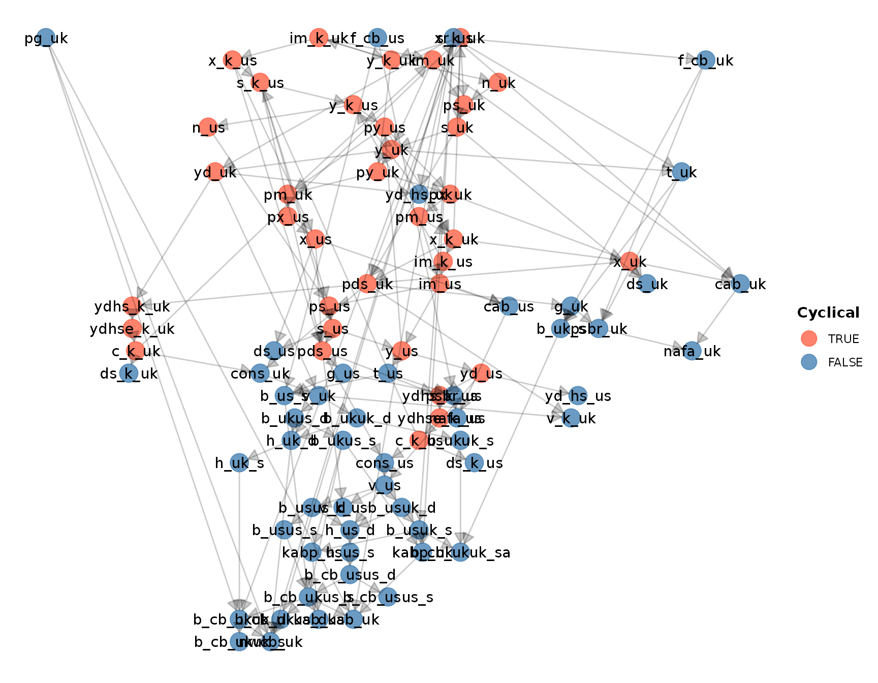
Sankey’s diagram: OPEN FIX
sfcr_sankey(tfm_openfix, openfix)Helper plot function
# (b_ukus_d_2/xr_us_2)/v_uk_2 b_ukus_d_2/v_uk_2
do_plot <- function(model, variables) {
model %>%
mutate(tab_uk = x_uk - im_uk,
tab_us = x_us - im_us,
gab_uk = -psbr_uk,
gab_us = -psbr_us,
dres_uk = b_cb_ukus_d - lag(b_cb_ukus_d),
db_cb_uk = b_cb_ukuk_d - lag(b_cb_ukuk_d),
dh_uk = h_uk_s - lag(h_uk_s),
dh_us = h_us_s - lag(h_us_s),
by_uk = b_uk_s / y_uk,
by_us = b_us_s / y_us,
bukus_p = (b_ukus_d/xr_us)/v_uk,
bukus_d = b_ukus_d / v_uk) %>%
pivot_longer(cols = -period) %>%
filter(name %in% variables) %>%
ggplot(aes(x = period, y = value)) +
geom_line(aes(linetype = name))
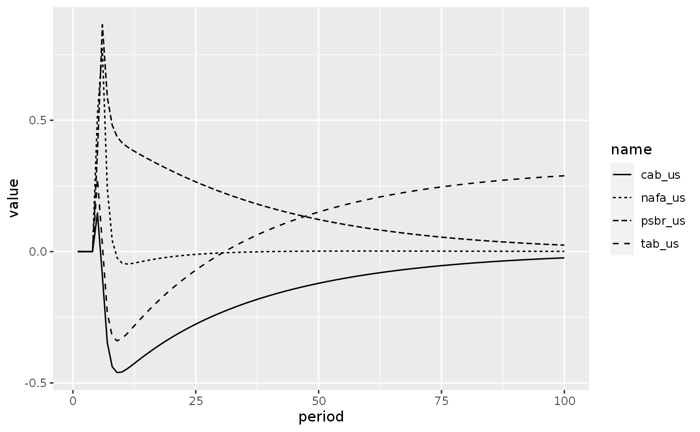
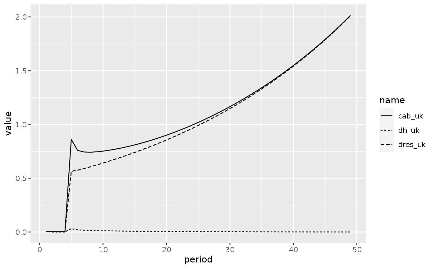
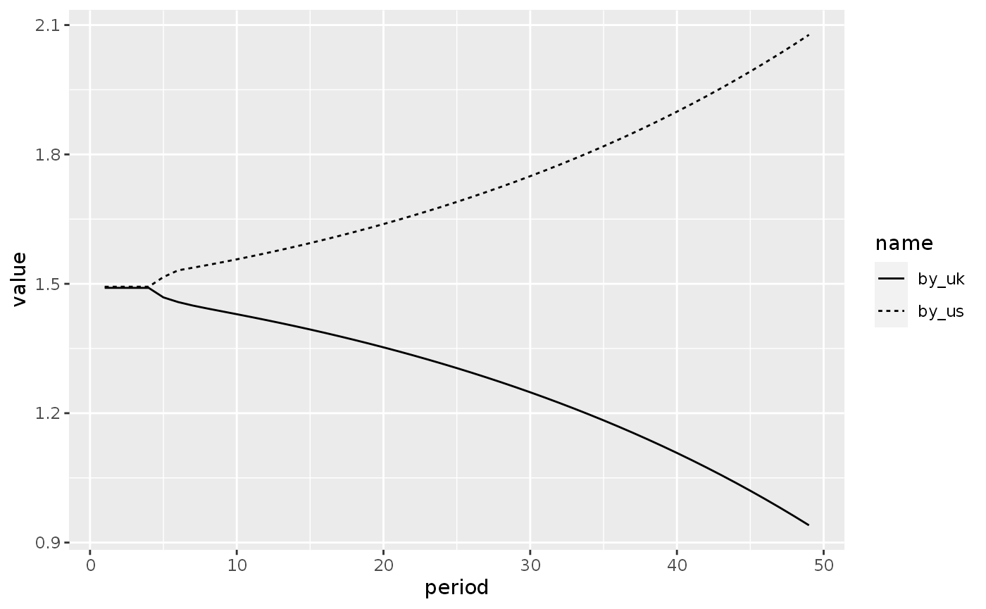
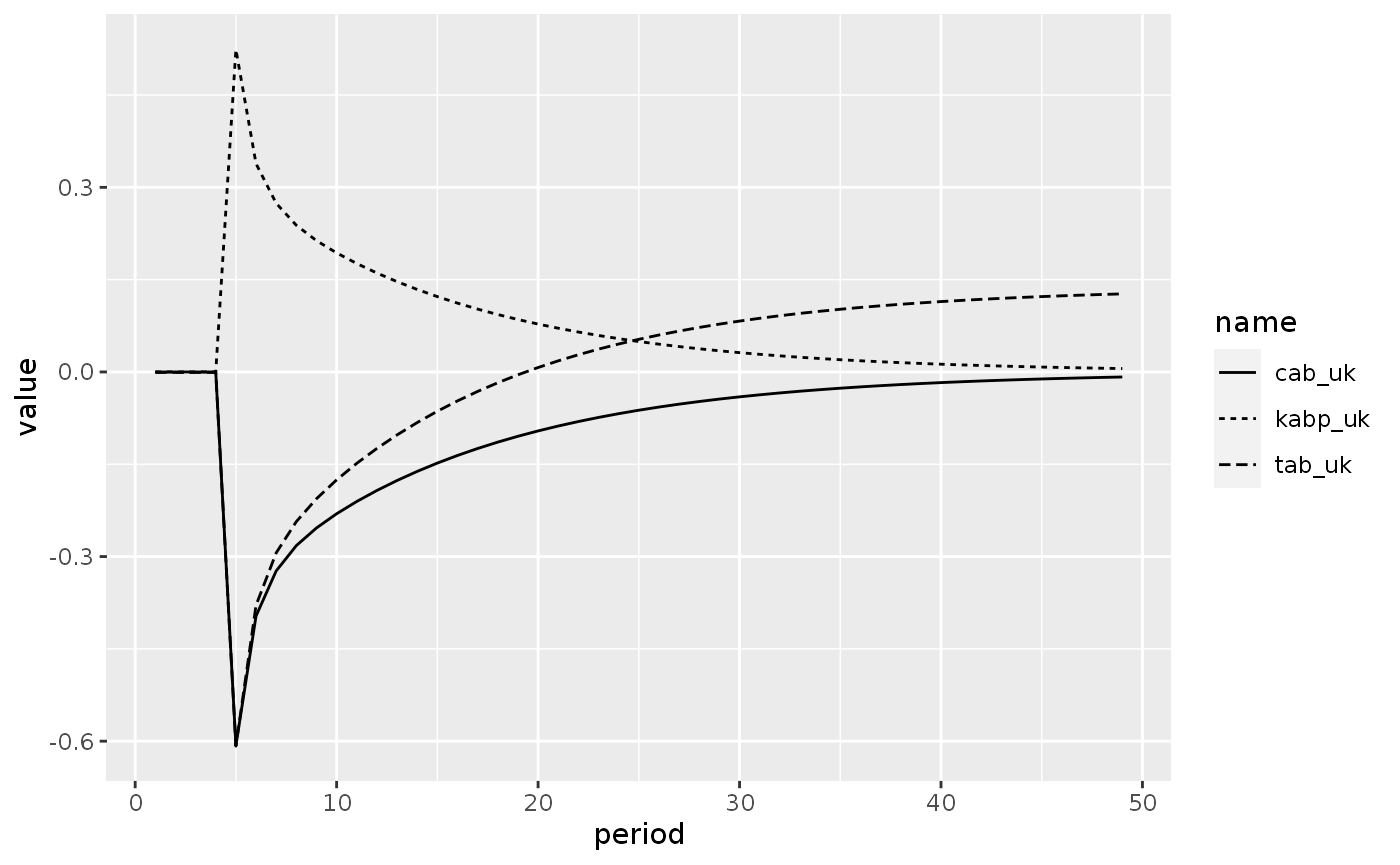
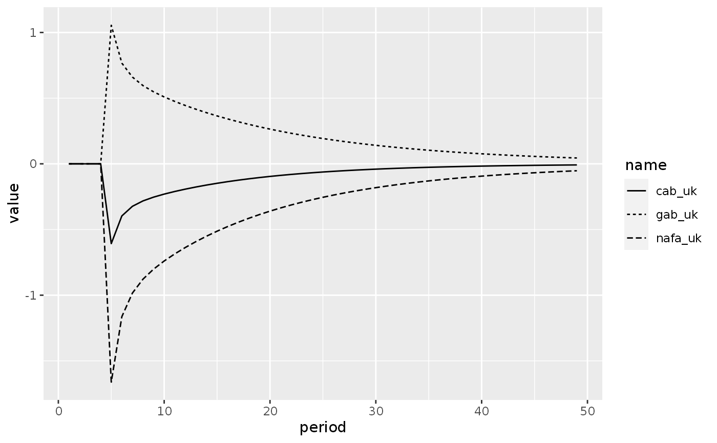
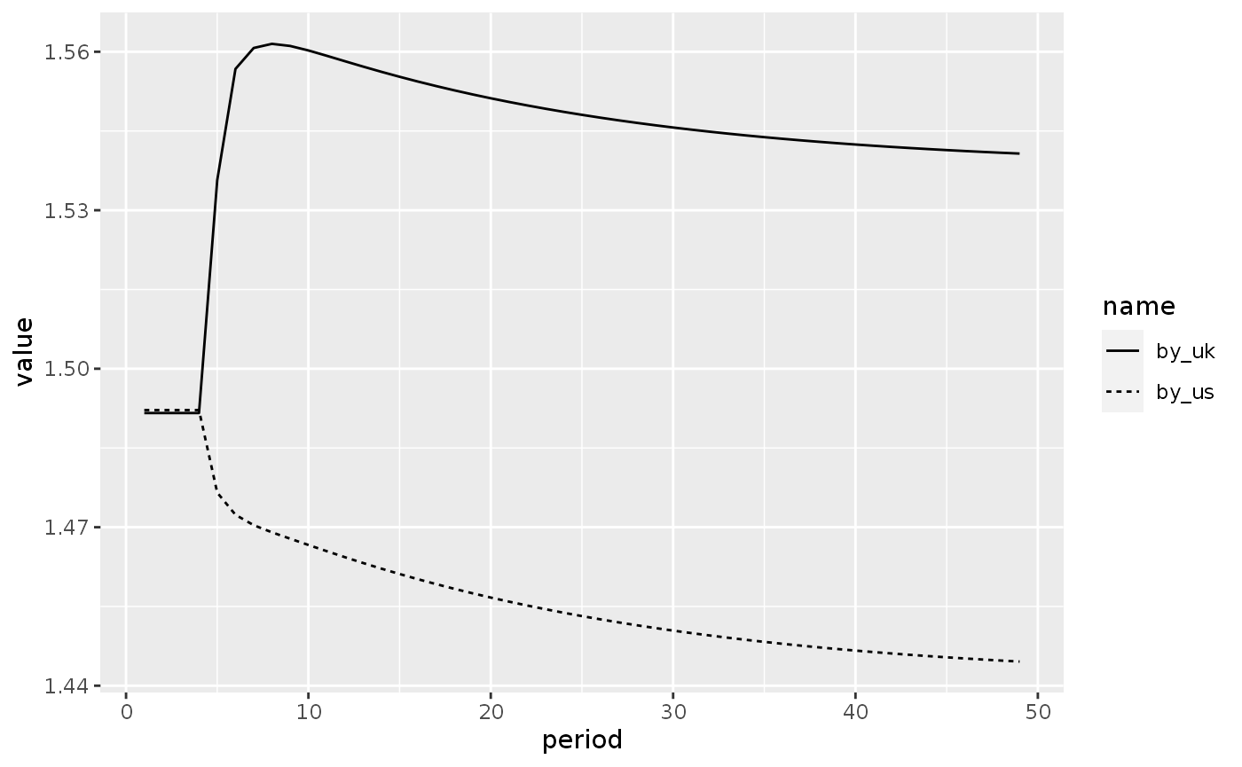
}Scenario 1: Increase in the US propensity to import
shock1 <- sfcr_shock(v = sfcr_set(eps0 ~ -2), s = 5, e = 100)
openfix1 <- sfcr_scenario(openfix, shock1, 100, method = "Broyden")
Figure 12.A
openfix1 %>%
  filter(period < 50) %>%
  do_plot(variables = c("cab_uk", "nafa_uk", "gab_uk", "tab_uk"))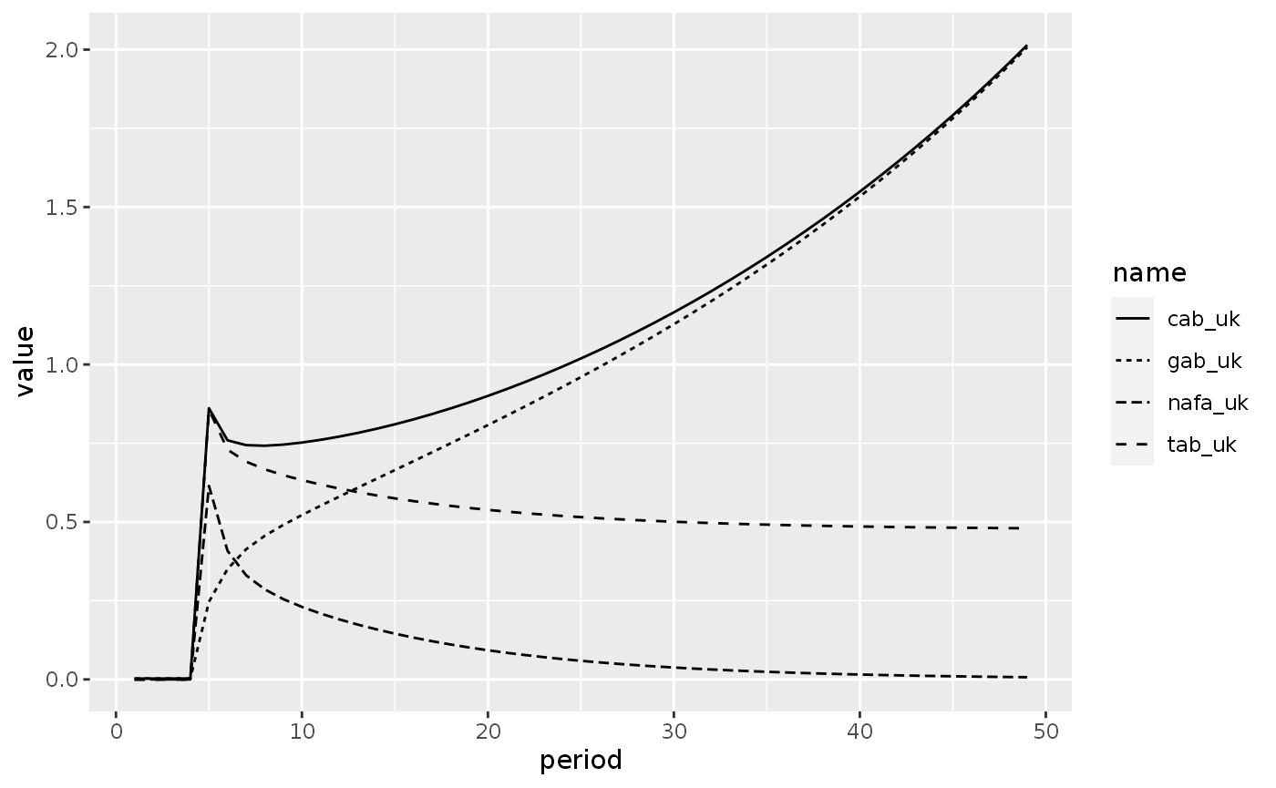
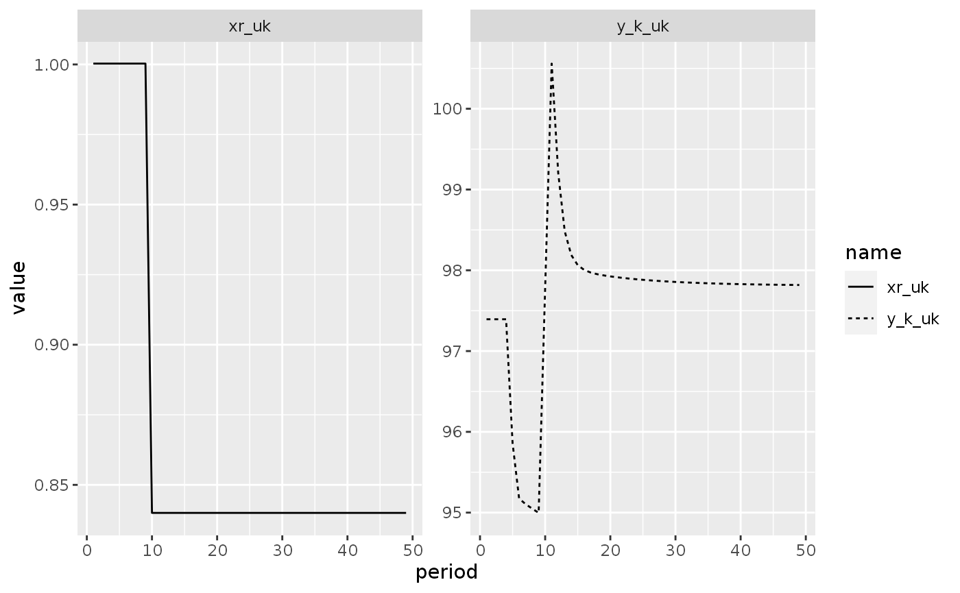
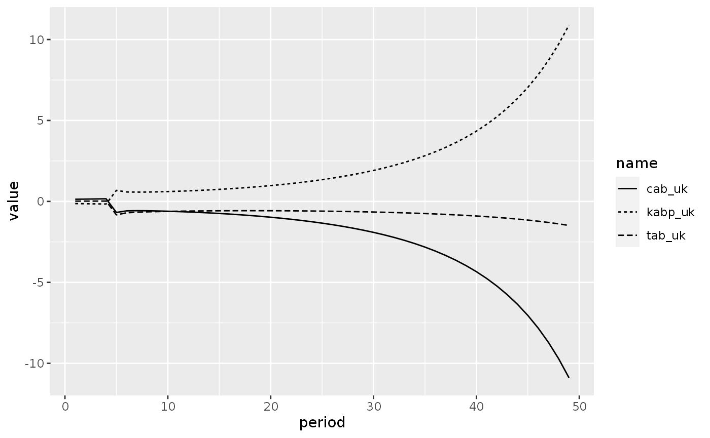
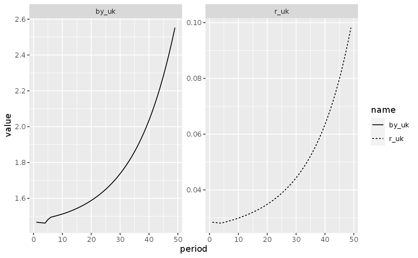
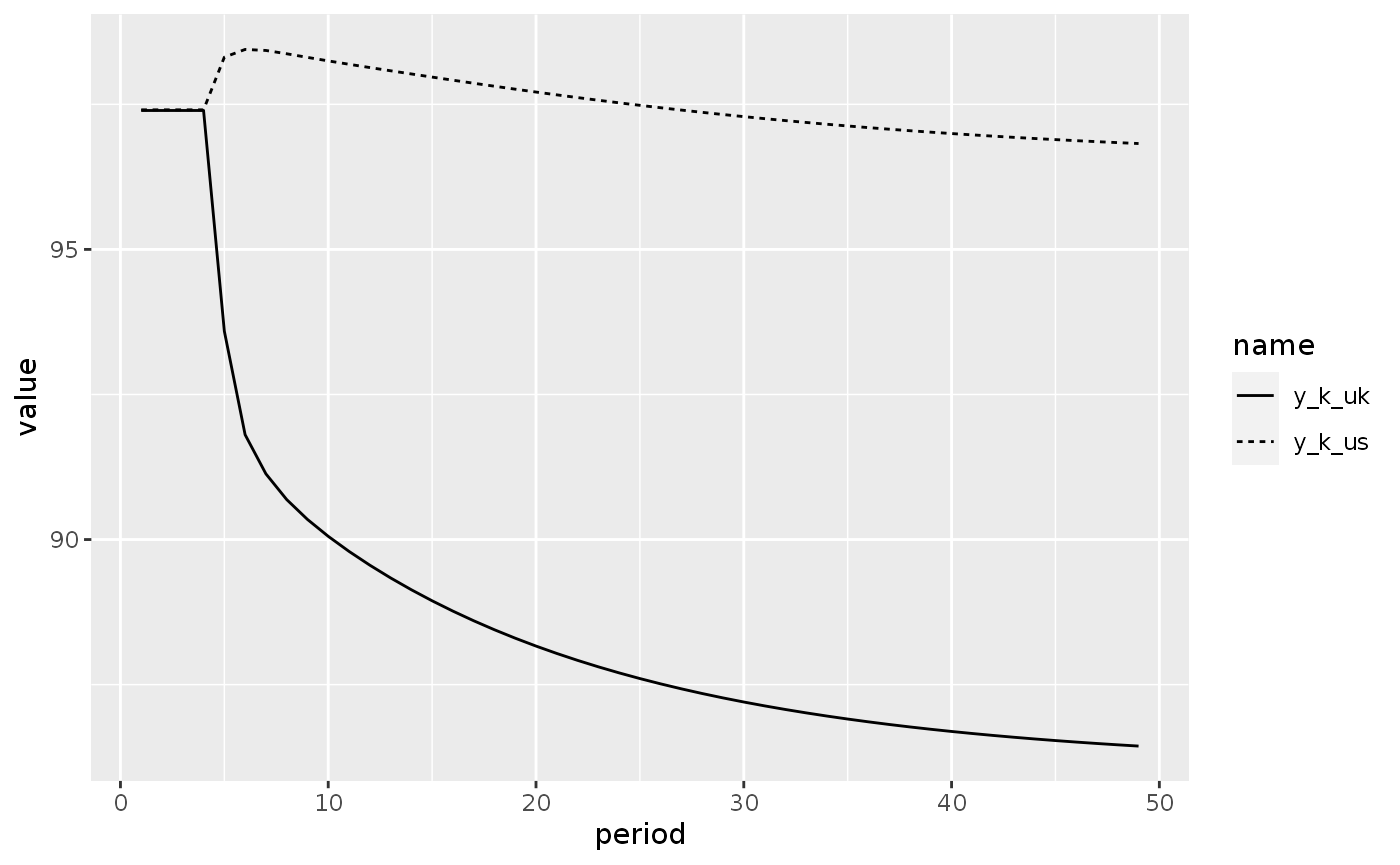
Scenario 2: A one-step devaluation after an increase in the UK propensity to import
shock2 <- sfcr_shock(v = sfcr_set(mu0 ~ -2), s = 5, e = 100)
shock3 <- sfcr_shock(v = sfcr_set(xr_uk ~ 0.84), s = 10, e = 100)
openfix2 <- sfcr_scenario(openfix, list(shock2, shock3), 100, method = "Broyden")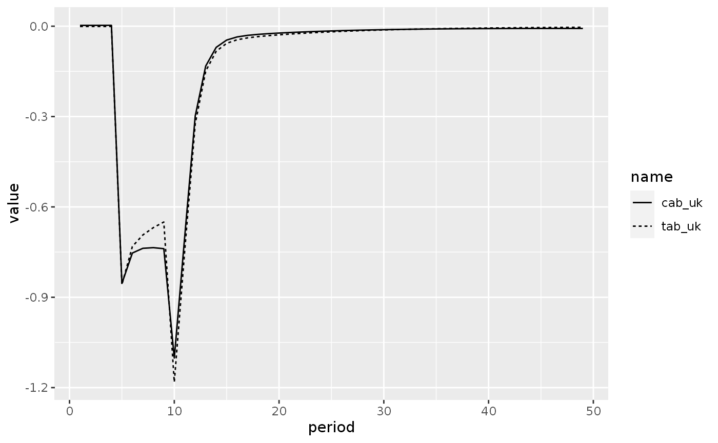
Model OPEN FIX R
Closure
# Find the equation to exclude
open12_eqs %>%
  sfcr_set_index() %>%
  filter(lhs == "b_ukus_d")
#> # A tibble: 1 × 3
#>      id lhs      rhs
#>   <int> <chr>    <chr>
#> 1    64 b_ukus_d v_uk * (lambda20 - lambda21 * r_uk + lambda22 * (r_us + dxre_u…

openfixr_eqs <- sfcr_set(
  open12_eqs,
  # 12.89R : Demand of UK Bills in US
  b_ukus_d ~ b_ukus_s*xr_us,
  # 12.90R : Supply of UK bills to us
  b_ukus_s ~  b_us_s - b_usus_s - b_cb_usus_d - b_cb_ukus_s,
  # 12.68R: Endogenous interest rate
  r_uk ~ (lambda20 + lambda22*(r_us + dxre_us) - b_ukus_d/v_uk)/lambda21,
  exclude = 64
)

openfixr_ext <- sfcr_set(
  open12_ext,
  # Eq. 12.91R
  xr_uk ~ 1.0003,
  b_cb_ukus_s ~ 0.02031
)
Baseline
openfixr <- sfcr_baseline(
  openfixr_eqs,
  openfixr_ext,
  periods = 100,
  initial = open12_init,
  method = "Broyden"
)
openfixr %>%
  select(b_cb_ukuk_s, b_cb_ukuk_sa)
#> # A tibble: 100 × 2
#>    b_cb_ukuk_s b_cb_ukuk_sa
#>          <dbl>        <dbl>
#>  1       0.280        0.280
#>  2       0.280        0.280
#>  3       0.280        0.280
#>  4       0.280        0.280
#>  5       0.280        0.280
#>  6       0.280        0.280
#>  7       0.280        0.280
#>  8       0.280        0.280
#>  9       0.280        0.280
#> 10       0.280        0.280
#> # … with 90 more rows
Scenario 1: Increase in the UK propensity to import
shock1 <- sfcr_shock(v = sfcr_set(mu0 ~ -2), s = 5, e = 100)

openfixr1 <- sfcr_scenario(
  openfixr, shock1, 100, method = "Broyden"
)
Model OPEN FIX G
Closure
# Find the equations to exclude

open12_eqs %>%
  sfcr_set_index() %>%
  filter(lhs %in% c("b_uk_s", "b_cb_ukuk_s", "g_uk"))
#> # A tibble: 3 × 3
#>      id lhs         rhs
#>   <int> <chr>       <chr>
#> 1    11 b_uk_s      b_uk_s[-1] + g_uk + r_uk[-1] * b_uk_s[-1] - t_uk - f_cb_uk
#> 2    59 g_uk        g_k_uk * pds_uk
#> 3    74 b_cb_ukuk_s b_cb_ukuk_d

open12_ext %>%
  sfcr_set_index() %>%
  filter(lhs %in% "g_k_uk")
#> # A tibble: 1 × 3
#>      id lhs    rhs
#>   <int> <chr>  <chr>
#> 1    32 g_k_uk 16

openfixg_eqs <- sfcr_set(
  open12_eqs,
  # 12.89G : Bills supply from UK to US
  b_ukus_s ~ xr_uk*b_ukus_d,
  # 12.90G : Supply of UK bills to us
  b_cb_ukus_s ~ b_us_s - b_usus_s - b_cb_usus_d - b_ukus_s,
  # 12.13G: Endogenous govt. expenditures in UK
  g_uk ~ b_uk_s - b_uk_s[-1] -(r_uk[-1]*b_uk_s[-1] - t_uk - f_cb_uk),
  # 12.61G: Real government expenditures
  g_k_uk ~ g_uk / pds_uk,
  # 12.82AG: Supply of UK Bills
  b_uk_s ~ b_usuk_s + b_ukuk_s + b_cb_ukuk_s,
  exclude = c(11, 59, 74)
)

openfixg_ext <- sfcr_set(
  open12_ext,
  # Eq. 12.91R
  xr_uk ~ 1.0003,
  r_uk ~ 0.03,
  b_cb_ukuk_s ~ 0.27984,
  exclude = 32
)
Baseline
openfixg <- sfcr_baseline(
  equations = openfixg_eqs,
  external = openfixg_ext,
  initial = open12_init,
  periods = 100,
  method = "Broyden",
)
#
Scenario 1
shock1 <- sfcr_shock(v = sfcr_set(mu0 ~ -2), s = 5, e = 100)

openfixg1 <- sfcr_scenario(
  openfixg, shock1, 100, method = "Broyden"
)
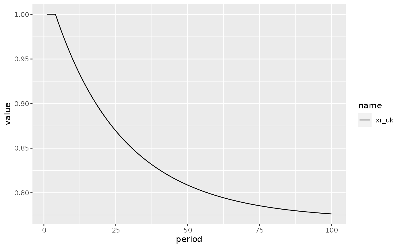
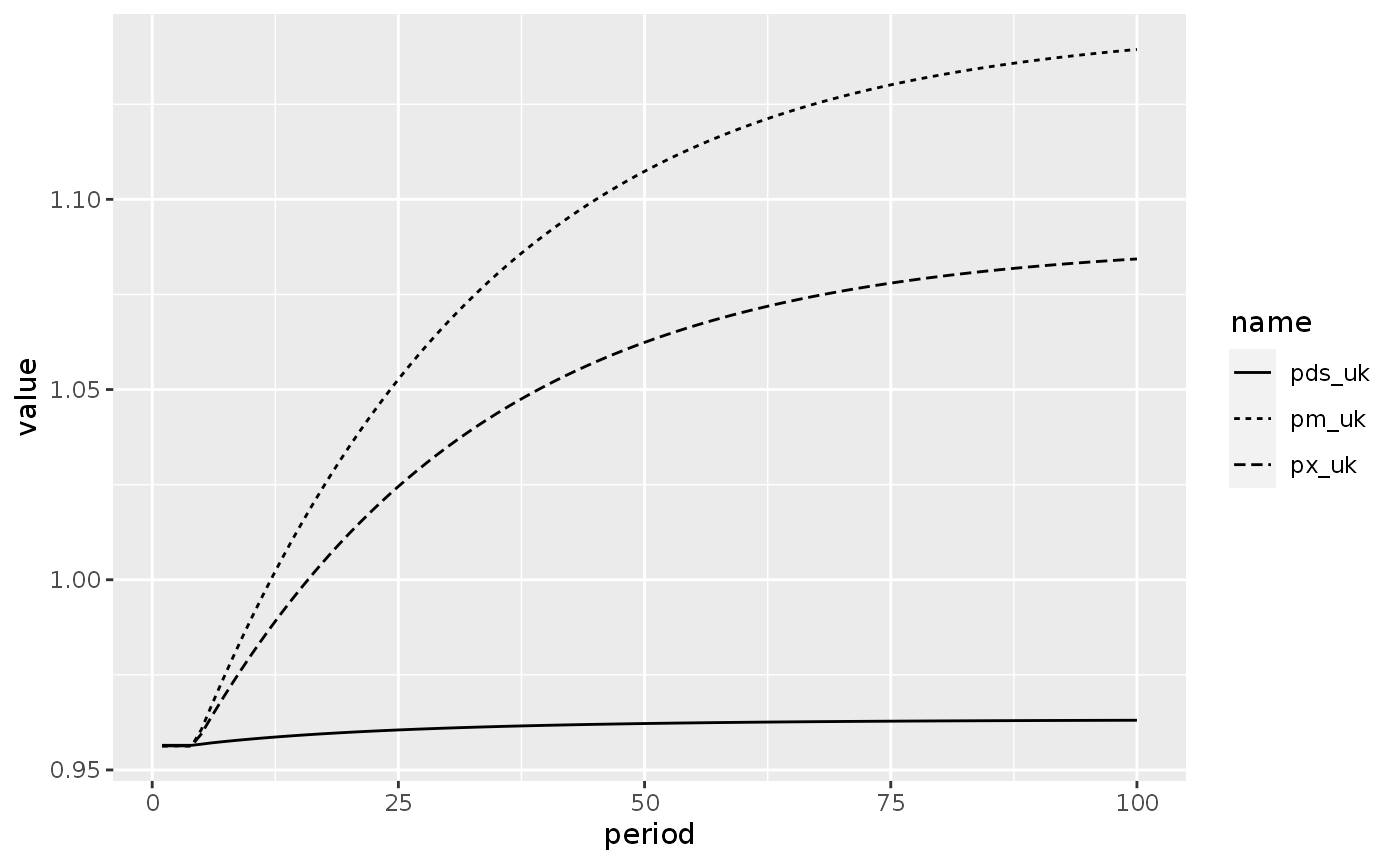
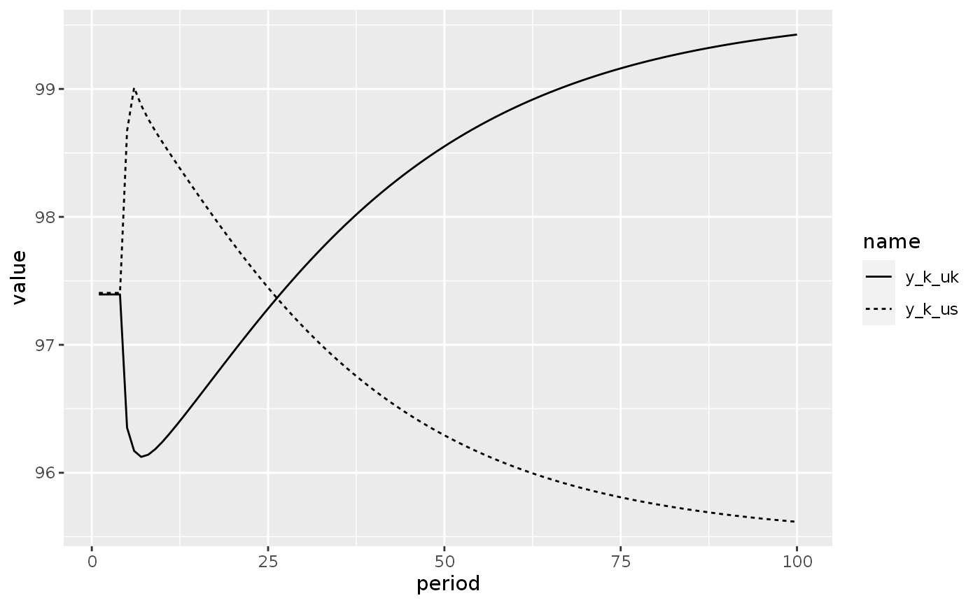
Model OPEN FLEX
Baseline
openflex <- sfcr_baseline(
equations = openflex_eqs,
external = openflex_ext,
initial = sfcr_set(open12_init),
periods = 100,
method = "Broyden",
hidden = c("b_cb_ukuk_s" = "b_cb_ukuk_sa")
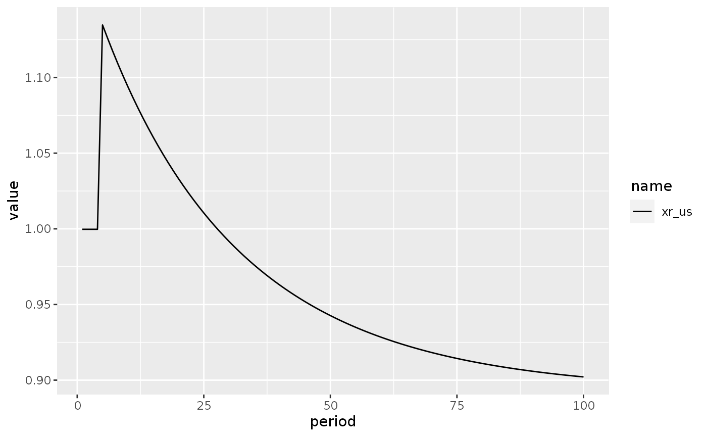
)Scenario 1: A decrease in the UK propensity to export
shock1 <- sfcr_shock(v = sfcr_set(eps0 ~ -2.2), s = 5, e = 100)
openflex1 <- sfcr_scenario(openflex, shock1, 100, method = "Broyden")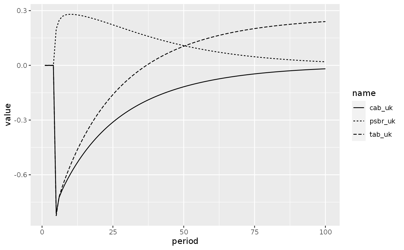
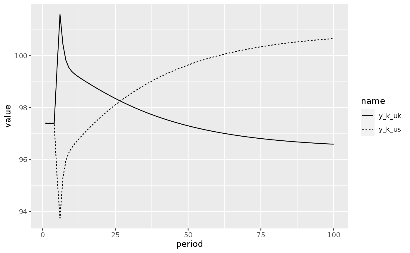
Scenario 2: A step increase in US government expenditures
shock2 <- sfcr_shock(v = sfcr_set(g_k_us ~ 18), s = 5, e = 100)
openflex2 <- sfcr_scenario(openflex, shock2, 100, method = "Broyden")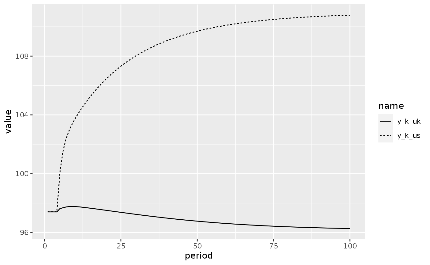
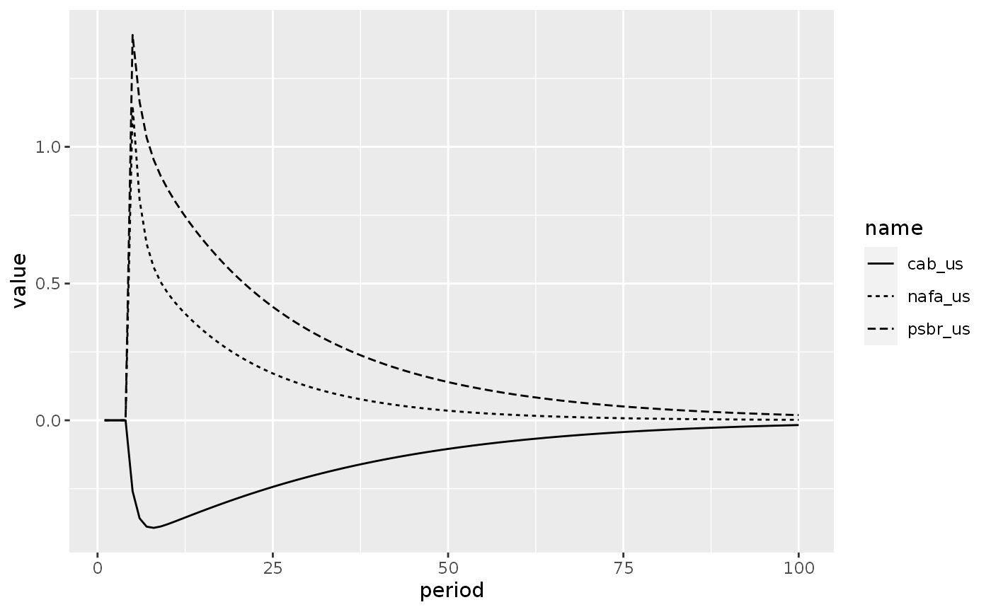
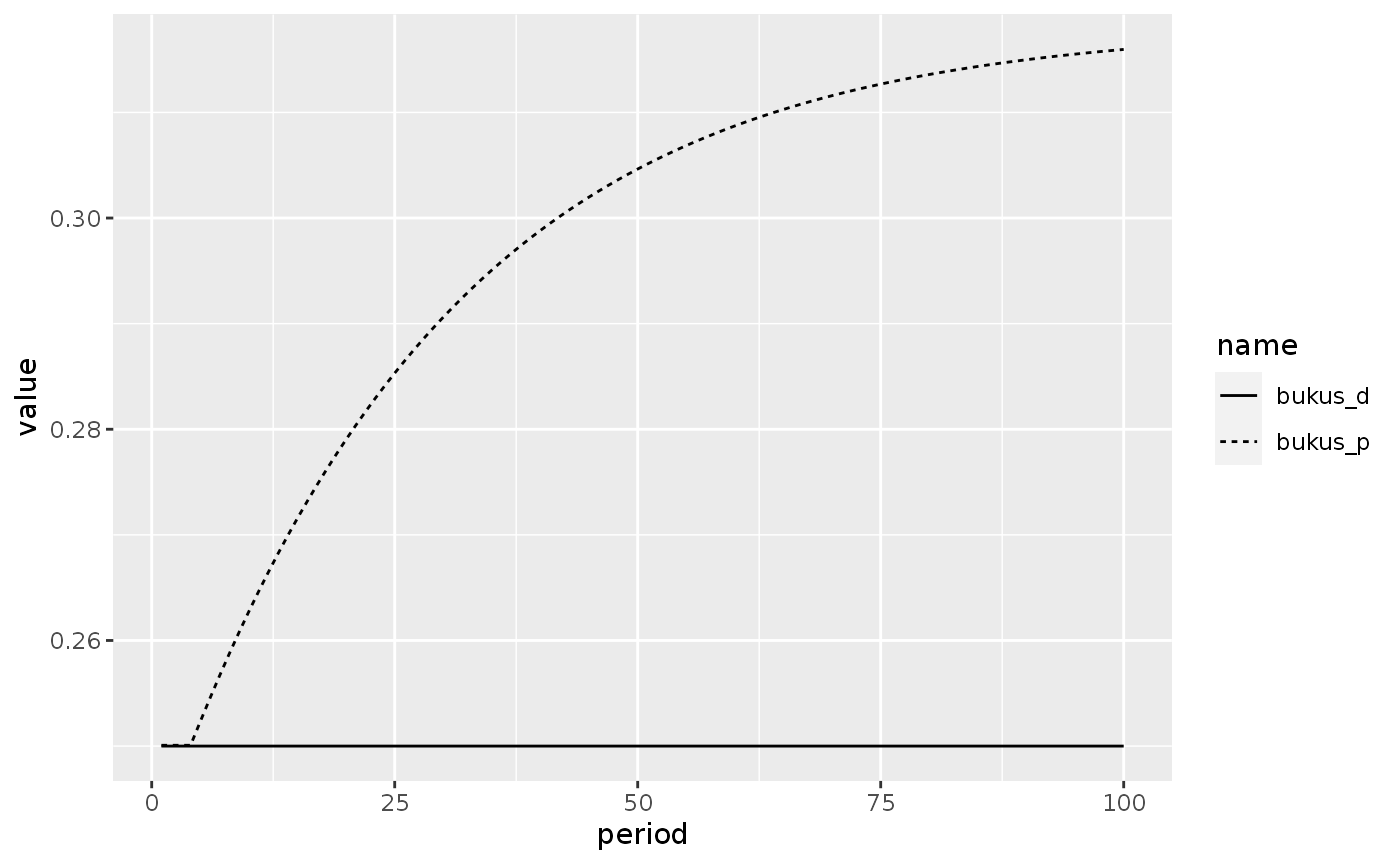
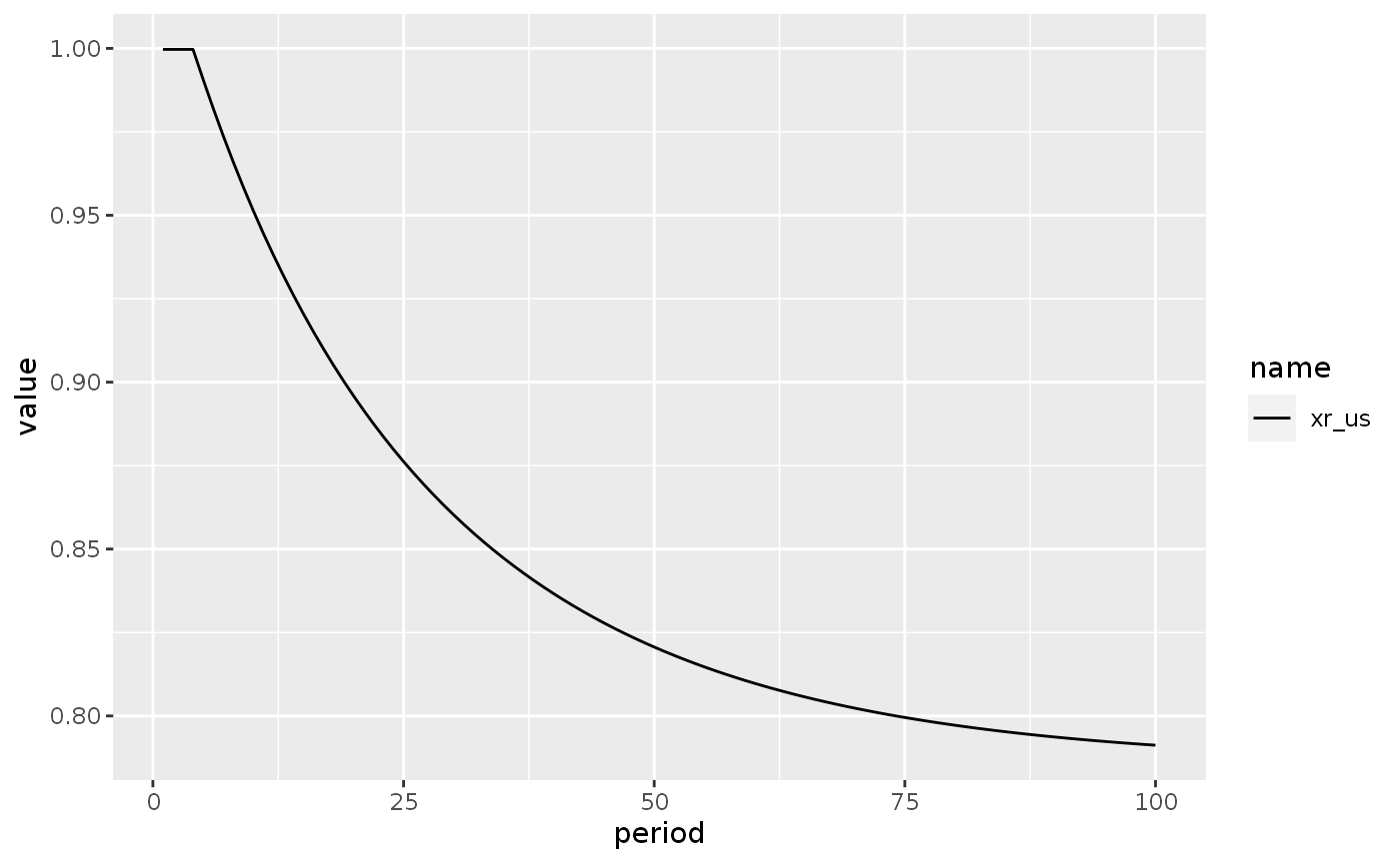
Scenario 3 - Increase in the desire to hold US treasury bills
shock3 <- sfcr_shock(v = sfcr_set(lambda20 ~ 0.30, lambda40 ~ 0.75), s = 5, e = 100)
openflex3 <- sfcr_scenario(openflex, shock3, 100, method = "Broyden")