library(sfcr)
library(tidyverse)
#> ── Attaching packages ─────────────────────────────────────── tidyverse 1.3.1 ──
#> ✔ ggplot2 3.3.5     ✔ purrr   0.3.4
#> ✔ tibble  3.1.5     ✔ dplyr   1.0.7
#> ✔ tidyr   1.1.4     ✔ stringr 1.4.0
#> ✔ readr   2.0.2     ✔ forcats 0.5.1
#> ── Conflicts ────────────────────────────────────────── tidyverse_conflicts() ──
#> ✖ dplyr::filter() masks stats::filter()
#> ✖ dplyr::lag()    masks stats::lag()

In this notebook I present the implementation of the GROWTH model from Godley and Lavoie (2007 ch. 11).

As a side note, I must say that this model is quite complicated to simulate, and I only could do it by using exactly the same equations as Zezza in his code, although some of the equations are different from the ones in the book. In this case, it means replicating exactly the same initial values in order to get a meaningful result.

Equations, parameters, and initial values

growth_eqs <- sfcr_set(
  Yk ~ Ske + INke - INk[-1],          # 11.1 : Real output
  Ske ~ beta*Sk + (1-beta)*Sk[-1]*(1 + (GRpr + RA)), # 11.2 : Expected real sales
  INke ~ INk[-1] + gamma*(INkt - INk[-1]),  # 11.3 : Long-run inventory target
  INkt ~ sigmat*Ske,                  # 11.4 : Short-run inventory target
  INk ~ INk[-1] + Yk - Sk - NPL/UC,   # 11.5 : Actual real inventories
  Kk ~ Kk[-1]*(1 + GRk),              # 11.6 : Real capital stock
  GRk ~ gamma0 + gammau*U[-1] - gammar*RRl,  # 11.7 : Growth of real capital stock
  U ~ Yk/Kk[-1],                      # 11.8 : Capital utilization proxy
  RRl ~ ((1 + Rl)/(1 + PI)) - 1,      # 11.9 : Real interest rate on loans
  PI ~ (P - P[-1])/P[-1],             # 11.10 : Rate of price inflation
  #Ik ~ (Kk - Kk[-1]) + delta*Kk[-1],          # 11.11 : Real gross investment
  Ik ~ (Kk - Kk[-1]) + delta * Kk[-1],

  # Box 11.2 : Firms equations
  # ---------------------------
  Sk ~ Ck + Gk + Ik,                  # 11.12 : Actual real sales
  S ~ Sk*P,                           # 11.13 : Value of realized sales
  IN ~ INk*UC,                        # 11.14 : Inventories valued at current cost
  INV ~ Ik*P,                         # 11.15 : Nominal gross investment
  K ~ Kk*P,                           # 11.16 : Nomincal value of fixed capital
  Y ~ Sk*P + (INk - INk[-1])*UC,               # 11.17 : Nomincal GDP

  # Box 11.3 : Firms equations
  # ---------------------------
  # 11.18 : Real wage aspirations
  omegat ~ exp(omega0 + omega1*log(PR) + omega2*log(ER + z3*(1 - ER) - z4*BANDt + z5*BANDb)),
  ER ~ N[-1]/Nfe[-1],                 # 11.19 : Employment rate
  # 11.20 : Switch variables
  z3a ~ if (ER > (1-BANDb)) {1} else {0},
  z3b ~ if (ER <= (1+BANDt)) {1} else {0},
  z3 ~  z3a * z3b,
  z4 ~ if (ER > (1+BANDt)) {1} else {0},
  z5 ~ if (ER < (1-BANDb)) {1} else {0},
  W ~ W[-1] + omega3*(omegat*P[-1] - W[-1]),  # 11.21 : Nominal wage
  PR ~ PR[-1]*(1 + GRpr),             # 11.22 : Labor productivity
  Nt ~ Yk/PR,                         # 11.23 : Desired employment
  N ~ N[-1] + etan*(Nt - N[-1]),      # 11.24 : Actual employment --> etan not in the book
  WB ~ N*W,                           # 11.25 : Nominal wage bill
  UC ~ WB/Yk,                         # 11.26 : Actual unit cost
  NUC ~ W/PR,                         # 11.27 : Normal unit cost
  NHUC ~ (1 - sigman)*NUC + sigman*(1 + Rln[-1])*NUC[-1],  # 11.28 : Normal historic unit cost

  # Box 11.4 : Firms equations
  # ---------------------------
  P ~ (1 + phi)*NHUC,                 # 11.29 : Normal-cost pricing
  phi ~ phi[-1] + eps2*(phit[-1] - phi[-1]),  # 11.30 : Actual mark-up --> eps2 not in the book
  # 11.31 : Ideal mark-up
  #phit ~ (FDf + FUft + Rl[-1]*(Lfd[-1] - IN[-1]))/((1 - sigmase)*Ske*UC + (1 + Rl[-1])*sigmase*Ske*UC[-1]),
  phit ~ (FUft + FDf + Rl[-1]*(Lfd[-1] - IN[-1])) / ((1 - sigmase)*Ske*UC + (1 + Rl[-1])*sigmase*Ske*UC[-1]),
  HCe ~ (1 - sigmase)*Ske*UC + (1 + Rl[-1])*sigmase*Ske*UC[-1],  # 11.32 : Expected historical costs
  sigmase ~ INk[-1]/Ske,              # 11.33 : Opening inventories to expected sales ratio
  Fft ~ FUft + FDf + Rl[-1]*(Lfd[-1] - IN[-1]),  # 11.34 : Planned entrepeneurial profits of firmss
  FUft ~ psiu*INV[-1],                # 11.35 : Planned retained earnings of firms
  FDf ~ psid*Ff[-1],                  # 11.36 : Dividends of firms

  # Box 11.5 : Firms equations
  # ---------------------------
  Ff ~ S - WB + (IN - IN[-1]) - Rl[-1]*IN[-1],  # 11.37 : Realized entrepeneurial profits
  FUf ~ Ff - FDf - Rl[-1]*(Lfd[-1] - IN[-1]) + Rl[-1]*NPL,  # 11.38 : Retained earnings of firms
  # 11.39 : Demand for loans by firms
  Lfd ~ Lfd[-1] + INV + (IN - IN[-1]) - FUf - (Eks - Eks[-1])*Pe - NPL,
  # NPL ~ NPLk*Lfs[-1],                 # 11.40 : Defaulted loans
  NPL ~ NPLk * Lfs[-1],
  Eks ~ Eks[-1] + ((1 - psiu)*INV[-1])/Pe,  # 11.41 : Supply of equities issued by firms
  # Rk ~ FDf/(Pe[-1]*Ekd[-1]),          # 11.42 : Dividend yield of firms
  Rk ~ FDf/(Pe[-1] * Ekd[-1]),
  PE ~ Pe/(Ff/Eks[-1]),               # 11.43 : Price earnings ratio
  Q ~ (Eks*Pe + Lfd)/(K + IN),        # 11.44 : Tobins Q ratio

  # Box 11.6 : Households equations
  # --------------------------------
  # YP ~ WB + FDf + FDb + Rm[-1]*Md[-1] + Rb[-1]*Bhd[-1] + BLs[-1],  # 11.45 : Personal income
  YP ~ WB + FDf + FDb + Rm[-1]*Mh[-1] + Rb[-1]*Bhd[-1] + BLs[-1],
  #YP ~ WB + FDf + FDb + Rm[-1]*Mh[-1] + Rb[-1]*Bhd[-1] + BLs[-1] + NL,
  TX ~ theta*YP,                       # 11.46 : Income taxes
  YDr ~ YP - TX - Rl[-1]*Lhd[-1],      # 11.47 : Regular disposable income
  YDhs ~ YDr + CG,                    # 11.48 : Haig-Simons disposable income
  # !1.49 : Capital gains
  CG ~ (Pbl - Pbl[-1])*BLd[-1] + (Pe - Pe[-1])*Ekd[-1] + (OFb - OFb[-1]),
  # 11.50 : Wealth
  V ~ V[-1] + YDr - CONS + (Pbl - Pbl[-1])*BLd[-1] + (Pe - Pe[-1])*Ekd[-1] + (OFb - OFb[-1]),
  Vk ~ V/P,                           # 11.51 : Real staock of wealth
  CONS ~ Ck*P,                        # 11.52 : Consumption
  Ck ~ alpha1*(YDkre + NLk) + alpha2*Vk[-1],  # 11.53 : Real consumption
  YDkre ~ eps*YDkr + (1 - eps)*(YDkr[-1]*(1 + GRpr)),  # 11.54 : Expected real regular disposable income
  # YDkr ~ YDr/P - (P - P[-1])*Vk[-1]/P,  # 11.55 : Real regular disposable income
  YDkr ~ YDr/P - ((P - P[-1]) * Vk[-1])/P,

  # Box 11.7 : Households equations
  # --------------------------------
  GL ~ eta*YDr,                       # 11.56 : Gross amount of new personal loans ---> new eta here
  eta ~ eta0 - etar*RRl,              # 11.57 : New loans to personal income ratio
  NL ~ GL - REP,                      # 11.58 : Net amount of new personal loans
  REP ~ deltarep*Lhd[-1],             # 11.59 : Personal loans repayments
  Lhd ~ Lhd[-1] + GL - REP,           # 11.60 : Demand for personal loans
  NLk ~ NL/P,                         # 11.61 : Real amount of new personal loans
  # BUR ~ (REP + Rl[-1]*Lhd[-1])/YDr[-1],  # 11.62 : Burden of personal debt
  BUR ~ (REP + Rl[-1] * Lhd[-1]) / YDr[-1],

  # Box 11.8 : Households equations - portfolio decisions
  # -----------------------------------------------------

  # 11.64 : Demand for bills
  
  # YDr/V
  
  #Md ~ Vfma[-1] * (lambda10 + lambda11*Rm[-1] - lambda12 * Rb[-1] - lambda13 * Rbl[-1] - lambda14 * Rk[-1] + lambda25 * (YP/V)),
  Bhd ~ Vfma[-1]*(lambda20 + lambda22*Rb[-1] - lambda21*Rm[-1] - lambda24*Rk[-1] - lambda23*Rbl[-1] - lambda25*(YDr/V)),
  # 11.65 : Demand for bonds
  BLd ~ Vfma[-1]*(lambda30 - lambda32*Rb[-1] - lambda31*Rm[-1] - lambda34*Rk[-1] + lambda33*Rbl[-1] - lambda35*(YDr/V))/Pbl,
  # 11.66 : Demand for equities - normalized to get the price of equitities
  Pe ~ Vfma[-1]*(lambda40 - lambda42*Rb[-1] - lambda41*Rm[-1] + lambda44*Rk[-1] - lambda43*Rbl[-1] - lambda45*(YDr/V))/Ekd,
  Mh ~ Vfma - Bhd - Pe*Ekd - Pbl*BLd + Lhd,  # 11.67 : Money deposits - as a residual
  Vfma ~ V - Hhd - OFb,               # 11.68 : Investible wealth
  VfmaA ~ Mh + Bhd + Pbl * BLd + Pe * Ekd,
  Hhd ~ lambdac*CONS,                 # 11.69 : Households demand for cash
  Ekd ~ Eks,                          # 11.70 : Stock market equilibrium

  # Box 11.9 : Governments equations
  # ---------------------------------
  G ~ Gk*P,                           # 11.71 : Pure government expenditures
  Gk ~ Gk[-1]*(1 + GRg),              # 11.72 : Real government expenditures
  PSBR ~ G + BLs[-1] + Rb[-1]*(Bbs[-1] + Bhs[-1]) - TX,  # 11.73 : Government deficit --> BLs[-1] missing in the book
  # 11.74 : New issues of bills
  Bs ~ Bs[-1] + G - TX - (BLs - BLs[-1])*Pbl + Rb[-1]*(Bhs[-1] + Bbs[-1]) + BLs[-1],
  GD ~ Bbs + Bhs + BLs*Pbl + Hs, # 11.75 : Government debt 

  # Box 11.10 : The Central banks equations
  # ----------------------------------------
  Fcb ~ Rb[-1]*Bcbd[-1],              # 11.76 : Central bank profits
  BLs ~ BLd,                          # 11.77 : Bonds are supplied on demand
  Bhs ~ Bhd,                          # 11.78 : Household bills supplied on demand
  Hhs ~ Hhd,                          # 11.79 : Cash supplied on demand --> Mistake on the book
  Hbs ~ Hbd,                          # 11.80 : Reserves supplied on demand
  Hs ~ Hbs + Hhs,                     # 11.81 : Total supply of cash
  Bcbd ~ Hs,                          # 11.82 : Central bankd 
  Bcbs ~ Bcbd,                        # 11.83 : Supply of bills to Central bank
  Rb ~ Rbbar,                         # 11.84 : Interest rate on bills set exogenously
  Rbl ~ Rb + ADDbl,                   # 11.85 : Long term interest rate
  Pbl ~ 1/Rbl,                        # 11.86 : Price of long-term bonds

  # Box 11.11 : Commercial Banks equations
  # ---------------------------------------
  Ms ~ Mh,                            # 11.87 : Bank deposits supplied on demand
  Lfs ~ Lfd,                          # 11.88 : Loans to firms supplied on demand
  Lhs ~ Lhd,                          # 11.89 : Personal loans supplied on demand
  Hbd ~ ro*Ms,                        # 11.90 Reserve requirements of banks
  # 11.91 : Bills supplied to banks
  Bbs ~ Bbs[-1] + (Bs - Bs[-1]) - (Bhs - Bhs[-1]) - (Bcbs - Bcbs[-1]),
  # 11.92 : Balance sheet constraint of banks
  Bbd ~ Ms + OFb - Lfs - Lhs - Hbd, 
  BLR ~ Bbd/Ms,                       # 11.93 : Bank liquidity ratio
  # 11.94 : Deposit interest rate
  Rm ~ Rm[-1] + z1a*xim1 + z1b*xim2 - z2a*xim1 - z2b*xim2,
  # 11.95-97 : Mechanism for determining changes to the interest rate on deposits
  z2a ~ if (BLR[-1] > (top + .05)) {1} else {0},
  z2b ~ if (BLR[-1] > top) {1} else {0},
  z1a ~ if (BLR[-1] <= bot) {1} else {0},
  z1b ~ if (BLR[-1] <= (bot -.05)) {1} else {0},

  # Box 11.12 : Commercial banks equations
  # ---------------------------------------
  Rl ~ Rm + ADDl,                     # 11.98 : Loan interest rate
  OFbt ~ NCAR*(Lfs[-1] + Lhs[-1]),    # 11.99 : Long-run own funds target
  OFbe ~ OFb[-1] + betab*(OFbt - OFb[-1]),  # 11.100 : Short-run own funds target
  FUbt ~ OFbe - OFb[-1] + NPLke*Lfs[-1],  # 11.101 : Target retained earnings of banks
  NPLke ~ epsb*NPLke[-1] + (1 - epsb)*NPLk[-1],  # 11.102 : Expected proportion of non-performaing loans
  # FDb ~ Fb - FUb,                     # 11.103 : Dividends of banks
  FDb ~ Fb - FUb,
  Fbt ~ lambdab*Y[-1] + (OFbe - OFb[-1] + NPLke*Lfs[-1]),  # 11.104 : Target profits of banks
  # 11.105 : Actual profits of banks
  Fb ~ Rl[-1]*(Lfs[-1] + Lhs[-1] - NPL) + Rb[-1]*Bbd[-1] - Rm[-1]*Ms[-1],
  # 11.106 : Lending mark-up over deposit rate
  ADDl ~ (Fbt - Rb[-1]*Bbd[-1] + Rm[-1]*(Ms[-1] - (1 - NPLke)*Lfs[-1] - Lhs[-1]))/((1 - NPLke)*Lfs[-1] + Lhs[-1]), # --> I added the lag term to Rm
  FUb ~ Fb - lambdab*Y[-1],           # 11.107 : Actual retained earnings
  OFb ~ OFb[-1] + FUb - NPL,          # 11.108 : Own funds of banks
  CAR ~ OFb/(Lfs + Lhs),
  
  Vf ~ IN + K - Lfd - Ekd * Pe,       # Firm's wealth (memo for matrices)
  #Vg ~ -Bs - BLs * Pbl,\
  Ls ~ Lfs + Lhs,                     # Loans supply (memo for matrices)
  
  )

growth_parameters = sfcr_set(
  alpha1 ~ 0.75,
  alpha2 ~ 0.064,
  beta ~ 0.5,
  betab ~ 0.4,
  gamma ~ 0.15,
  gamma0 ~ 0.00122,
  gammar ~ 0.1,
  gammau ~ 0.05,
  delta ~ 0.10667,
  deltarep ~ 0.1,
  eps ~ 0.5,
  eps2 ~ 0.8,
  epsb ~ 0.25,
  epsrb ~ 0.9,
  eta0 ~ 0.07416,
  etan ~ 0.6,
  etar ~ 0.4,
  theta ~ 0.22844,
  # lambda10 ~ -0.17071,
  # lambda11 ~ 0,
  # lambda12 ~ 0,
  # lambda13 ~ 0,
  # lambda14 ~ 0,
  # lambda15 ~ 0.18,
  lambda20 ~ 0.25,
  lambda21 ~ 2.2,
  lambda22 ~ 6.6,
  lambda23 ~ 2.2,
  lambda24 ~ 2.2,
  lambda25 ~ 0.1,
  lambda30 ~ -0.04341,
  lambda31 ~ 2.2,
  lambda32 ~ 2.2,
  lambda33 ~ 6.6,
  lambda34 ~ 2.2,
  lambda35 ~ 0.1,
  lambda40 ~ 0.67132,
  lambda41 ~ 2.2,
  lambda42 ~ 2.2,
  lambda43 ~ 2.2,
  lambda44 ~ 6.6,
  lambda45 ~ 0.1,
  lambdab ~ 0.0153,
  lambdac ~ 0.05,
  xim1 ~ 0.0008,
  xim2 ~ 0.0007,
  ro ~ 0.05,
  sigman ~ 0.1666,
  sigmat ~ 0.2,
  psid ~ 0.15255,
  psiu ~ 0.92,
  omega0 ~ -0.20594,
  omega1 ~ 1,
  omega2 ~ 2,
  omega3 ~ 0.45621,
  
  # Exogenous
  
  ADDbl ~ 0.02,
  BANDt ~ 0.01,
  BANDb ~ 0.01,
  bot ~ 0.05,
  GRg ~ 0.03,
  GRpr ~ 0.03,
  Nfe ~ 87.181,
  NCAR ~ 0.1,
  NPLk ~ 0.02,
  Rbbar ~ 0.035,
  Rln ~ 0.07,
  RA ~ 0,
  top ~ 0.12,
  
  # sigmase ~ 0.16667,
  # eta ~ 0.04918,
  # phi ~ 0.26417,
  # phit ~ 0.26417,
  
  )


growth_initial <- sfcr_set(
  sigmase ~ 0.16667,
  eta ~ 0.04918,
  phi ~ 0.26417,
  phit ~ 0.26417,
  
  ADDbl ~ 0.02,
  BANDt ~ 0.01,
  BANDb ~ 0.01,
  bot ~ 0.05,
  GRg ~ 0.03,
  GRpr ~ 0.03,
  Nfe ~ 87.181,
  NCAR ~ 0.1,
  NPLk ~ 0.02,
  Rbbar ~ 0.035,
  Rln ~ 0.07,
  RA ~ 0,
  top ~ 0.12,
  
  
  ADDl ~ 0.04592,
  BLR ~ 0.1091,
  BUR ~ 0.06324,
  Ck ~ 7334240,
  CAR ~ 0.09245,
  CONS ~ 52603100,
  ER ~ 1,
  Fb ~ 1744130,
  Fbt ~ 1744140,
  Ff ~ 18081100,
  Fft ~ 18013600,
  FDb ~ 1325090,
  FDf ~ 2670970,
  FUb ~ 419039,
  FUf ~ 15153800,
  FUft ~ 15066200,
  G ~ 16755600,
  Gk ~ 2336160,
  GL ~ 2775900,
  GRk ~ 0.03001,
  INV ~ 16911600,
  Ik ~ 2357910,
  N ~ 87.181,
  Nt ~ 87.181,
  NHUC ~ 5.6735,
  NL ~ 683593,
  NLk ~ 95311,
  NPL ~ 309158,
  NPLke ~ 0.02,
  NUC ~ 5.6106,
  omegat ~ 112852,
  P ~ 7.1723,
  Pbl ~ 18.182,
  Pe ~ 17937,
  PE ~ 5.07185,
  PI ~ 0.0026,
  PR ~ 138659,
  PSBR ~ 1894780,
  Q ~ 0.77443,
  Rb ~ 0.035,
  Rbl ~ 0.055,
  Rk ~ 0.03008,
  Rl ~ 0.06522,
  Rm ~ 0.0193,
  REP ~ 2092310,
  #RRb ~ 0.03232,
  RRl ~ 0.06246,
  S ~ 86270300,
  Sk ~ 12028300,
  Ske ~ 12028300,
  TX ~ 17024100,
  U ~ 0.70073,
  UC ~ 5.6106,
  W ~ 777968,
  WB ~ 67824000,
  Y ~ 86607700,
  Yk ~ 12088400,
  YDr ~ 56446400,
  YDkr ~ 7813270,
  YDkre ~ 7813290,
  YP ~ 73158700,
  z1a ~ 0,
  z1b ~ 0,
  z2a ~ 0,
  z2b ~ 0,
  
  ##
  
  #Bbd ~ 4388930,
  #Bbs ~ 4388930,
  Bbd ~ 4389790,
  Bbs ~ 4389790,
  Bcbd ~ 4655690,
  Bcbs ~ 4655690,
  Bhd ~ 33439320,
  Bhs ~ 33439320,
  #Bhd ~ 33396900,
  #Bhs ~ 33396900,
  Bs ~ 42484800,
  #Bs ~ 42441520,
  BLd ~ 840742,
  BLs ~ 840742,
  GD ~ 57728700,
  Ekd ~ 5112.6001,
  Eks ~ 5112.6001,
  Hbd ~ 2025540,
  Hbs ~ 2025540,
  Hhd ~ 2630150,
  Hhs ~ 2630150,
  Hs ~ 4655690,
  IN ~ 11585400,
  INk ~ 2064890,
  INke ~ 2405660,
  INkt ~ 2064890,
  #K ~ 127444000,
  K ~ 127486471,
  #Kk ~ 17768900,
  Kk ~ 17774838,
  Lfd ~ 15962900,
  Lfs ~ 15962900,
  Lhd ~ 21606600,
  Lhs ~ 21606600,
  Ls ~ 37569500,
  #Md ~ 40510800,
  Mh ~ 40510800,
  Ms ~ 40510800,
  OFb ~ 3474030,
  OFbe ~ 3474030,
  #OFb ~ 3473280,
  #OFbe ~ 3782430,
  OFbt ~ 3638100,
  #V ~ 165395000,
  V ~ 165438779,
  #Vfma ~ 159291000,
  Vfma ~ 159334599,
  Vk ~ 23066350,
  Vf ~ 31361792
  
  )

Model GROWTH: Baseline

growth <- sfcr_baseline(
  equations = growth_eqs,
  external = growth_parameters,
  initial = growth_initial,
  periods = 350,
  method = "Broyden",
  hidden = c("Bbs" = "Bbd"),
  tol = 1e-15,
  max_iter = 350,
  rhtol = TRUE,
  .hidden_tol = 1e-6
)

The hidden equation: is it fulfilled?

In this model we can observe an interesting development: the hidden equation is not exactly fulfilled. In fact, the discrepancy between Bbs and Bbd is quite insignificant in the first period, but this discrepancy increases together with the stocks of the model. Therefore, we must set rhtol to TRUE in order to check that discrepancy between the two series as a share of the first series is always smaller than the .hidden_tol value.

To see if the model arrived to a stable steady state, let’s plot some key ratios and variables. As always, we first create a helper function to simplify the plotting procedure:

do_plot <- function(model, variables, plot = NULL) {
  m1 <- model %>%
    mutate(
      uk = Y / K,
      Bsk = Bs / K,
      VK = V / K,
      wi = (W - lag(W)) / lag(W),
      DefY = PSBR/Y,
      GDY = GD/Y,
      LIN = Lfd / IN,
      GRy = (Yk / lag(Yk)) - 1,
      LhYDr = Lhd / YDr,
      FUfInv = FUf / INV,
      EqFMA = (Pe * Ekd) / Vfma,
      GRFfk = -1 + (Ff / P)/(lag(Ff)/lag(P)),
      GRPek = -1 + (Pe / P) / (lag(Pe)/lag(P))) %>%
    pivot_longer(cols = c(-period))
  
  if (is.null(plot)) {
    m2 <- filter(m1, name %in% variables)
  }
  else {
    m2 <- filter(m1, name %in% plot)
  }
  
  m2 %>%
    ggplot(aes(x = period, y = value)) +
    geom_line(aes(linetype = name))
}

Steady state

growth %>%
  do_plot(variables = c("Uk", "Bsk", "VK", 'GRk', "PI")) +
    facet_wrap(~name, scales = "free_y")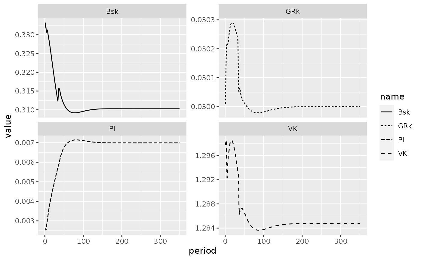

As we can see, the hidden equation is fulfilled (up to certain amount of computational error), key ratios and growth rations are stable. We can now check the balance-sheet and the transactions-flow matrices:

Matrices of model GROWTH

Balance-sheet matrix

bs_growth <- sfcr_matrix(
  columns = c("Households", "Firms", "Govt", "Central Bank", "Banks", "Sum"),
  codes = c("h", "f", "g", "cb", "b", "s"),
  c("Inventories", f = "+IN", s = "+IN"),
  c("Fixed Capital", f = "+K", s = "+K"),
  c("HPM", h = "+Hhd", cb = "-Hs", b = "+Hbd"),
  c("Money", h = "+Mh", b = "-Ms"),
  c("Bills", h = "+Bhd", g = "-Bs", cb = "+Bcbd", b = "+Bbd"),
  c("Bonds", h = "+BLd * Pbl", g = "-BLs * Pbl"),
  c("Loans", h = "-Lhd", f = "-Lfd", b = "+Ls"),
  c("Equities", h = "+Ekd * Pe", f = "-Eks * Pe"),
  c("Bank capital", h = "+OFb", b = "-OFb"),
  c("Balance", h = "-V", f = "-Vf", g = "GD", s = "-(IN + K)")
)

sfcr_matrix_display(bs_growth, which = "bs")

	Households	Firms	Govt	Central Bank	Banks	\(\sum\)
Inventories		\(+IN\)				\(+IN\)
Fixed Capital		\(+K\)				\(+K\)
HPM	\(+Hhd\)			\(-Hs\)	\(+Hbd\)	\(0\)
Money	\(+Mh\)				\(-Ms\)	\(0\)
Bills	\(+Bhd\)		\(-Bs\)	\(+Bcbd\)	\(+Bbd\)	\(0\)
Bonds	\(+BLd\cdot Pbl\)		\(-BLs\cdot Pbl\)			\(0\)
Loans	\(-Lhd\)	\(-Lfd\)			\(+Ls\)	\(0\)
Equities	\(+Ekd\cdot Pe\)	\(-Eks\cdot Pe\)				\(0\)
Bank capital	\(+OFb\)				\(-OFb\)	\(0\)
Balance	\(-V\)	\(-Vf\)	\(GD\)			\(-(IN+K)\)
\(\sum\)	\(0\)	\(0\)	\(0\)	\(0\)	\(0\)	\(0\)

Next we validate the model with the data:

sfcr_validate(bs_growth, growth, "bs", rtol = TRUE, tol = 1e-8)
#> Water tight! The balance-sheet matrix is consistent with the simulated model.

Transactions-flow matrix

tfm_growth <- sfcr_matrix(
  columns = c("Households", "Firms curr.", "Firms cap.", "Govt.", "CB curr.", "CB cap.", "Banks curr.", "Banks cap."),
  code = c("h", "fc", "fk", "g", "cbc", "cbk", "bc", "bk"),
  c("Consumption", h = '-CONS', fc = "+CONS"),
  c("Govt. Exp.", fc = "+G", g = "-G"),
  c("Investment", fc = "+INV", fk = "-INV"),
  c("Inventories", fc = "+(IN - IN[-1])", fk = "-(IN - IN[-1])"),
  c("Taxes", h = "-TX", g = "+TX"),
  c("Wages", h = "+WB", fc = "-WB"),
  c("Inventory financing cost", fc = "-Rl[-1] * IN[-1]", bc = "+Rl[-1] * (IN[-1])"),
  c("Entr. Profits", h = "+FDf", fc = "-Ff", fk = "+FUf", bc = "+Rl[-1] * (Lfs[-1] - IN[-1] - NPL)"),
  c("Banks Profits", h = "+FDb", bc = "-Fb", bk = "+FUb"),
  # Interests
  c("Int. hh loans", h = "-Rl[-1] * Lhd[-1]", bc = "+Rl[-1] * Lhs[-1]"),
  c("Int. deposits", h = "+Rm[-1] * Mh[-1]", bc = "-Rm[-1] * Ms[-1]"),
  c("Int. bills", h = "+Rb[-1] * Bhd[-1]", g = "-Rb[-1] * Bs[-1]", cbc = "+Rb[-1] * Bcbd[-1]", bc = "+Rb[-1] * Bbd[-1]"),
  c("Int. bonds", h = "+BLd[-1]", g = "-BLd[-1]"),
  # Change in stocks
  c("Ch. loans", h = "+(Lhd - Lhd[-1])", fk = "+(Lfd - Lfd[-1])", bk = "-(Ls - Ls[-1])"),
  c("Ch. cash", h = "-(Hhd - Hhd[-1])", cbk = "+(Hs - Hs[-1])", bk = "-(Hbd - Hbd[-1])"),
  c("Ch. deposits", h = "-(Mh - Mh[-1])", bk = "+(Ms - Ms[-1])"),
  c("Ch. bills", h = "-(Bhd - Bhd[-1])", g = "+(Bs - Bs[-1])", cbk = "-(Bcbd - Bcbd[-1])", bk = "-(Bbd - Bbd[-1])"),
  c("Ch. bonds", h = "-(BLd - BLd[-1]) * Pbl", g = "+(BLs - BLs[-1]) * Pbl"),
  c("Ch. equities", h = "-(Ekd - Ekd[-1]) * Pe", fk = "+(Eks - Eks[-1]) * Pe"),
  # Loan defaults
  c("Loan defaults", fk = "+NPL", bk = "-NPL")
)

sfcr_matrix_display(tfm_growth, "tfm")

	Households	Firms curr.	Firms cap.	Govt.	CB curr.	CB cap.	Banks curr.	Banks cap.	\(\sum\)
Consumption	\(-CONS\)	\(+CONS\)							\(0\)
Govt. Exp.		\(+G\)		\(-G\)					\(0\)
Investment		\(+INV\)	\(-INV\)						\(0\)
Inventories		\(+\Delta IN\)	\(-\Delta IN\)						\(0\)
Taxes	\(-TX\)			\(+TX\)					\(0\)
Wages	\(+WB\)	\(-WB\)							\(0\)
Inventory financing cost		\(-Rl_{-1}\cdot IN_{-1}\)					\(+Rl_{-1}\cdot (IN_{-1})\)		\(0\)
Entr. Profits	\(+FDf\)	\(-Ff\)	\(+FUf\)				\(+Rl_{-1}\cdot (Lfs_{-1}-IN_{-1}-NPL)\)		\(0\)
Banks Profits	\(+FDb\)						\(-Fb\)	\(+FUb\)	\(0\)
Int. hh loans	\(-Rl_{-1}\cdot Lhd_{-1}\)						\(+Rl_{-1}\cdot Lhs_{-1}\)		\(0\)
Int. deposits	\(+Rm_{-1}\cdot Mh_{-1}\)						\(-Rm_{-1}\cdot Ms_{-1}\)		\(0\)
Int. bills	\(+Rb_{-1}\cdot Bhd_{-1}\)			\(-Rb_{-1}\cdot Bs_{-1}\)	\(+Rb_{-1}\cdot Bcbd_{-1}\)		\(+Rb_{-1}\cdot Bbd_{-1}\)		\(0\)
Int. bonds	\(+BLd_{-1}\)			\(-BLd_{-1}\)					\(0\)
Ch. loans	\(+\Delta Lhd\)		\(+\Delta Lfd\)					\(-\Delta Ls\)	\(0\)
Ch. cash	\(-\Delta Hhd\)					\(+\Delta Hs\)		\(-\Delta Hbd\)	\(0\)
Ch. deposits	\(-\Delta Mh\)							\(+\Delta Ms\)	\(0\)
Ch. bills	\(-\Delta Bhd\)			\(+\Delta Bs\)		\(-\Delta Bcbd\)		\(-\Delta Bbd\)	\(0\)
Ch. bonds	\(-\Delta BLd\cdot Pbl\)			\(+\Delta BLs\cdot Pbl\)					\(0\)
Ch. equities	\(-\Delta Ekd\cdot Pe\)		\(+\Delta Eks\cdot Pe\)						\(0\)
Loan defaults			\(+NPL\)					\(-NPL\)	\(0\)
\(\sum\)	\(0\)	\(0\)	\(0\)	\(0\)	\(0\)	\(0\)	\(0\)	\(0\)	\(0\)

And we validate the model with the data:

sfcr_validate(tfm_growth, growth, "tfm", tol = 1e-7, rtol = TRUE)
#> Water tight! The transactions-flow matrix is consistent with the simulated model.

Sankey’s diagram:

sfcr_sankey(tfm_growth, growth)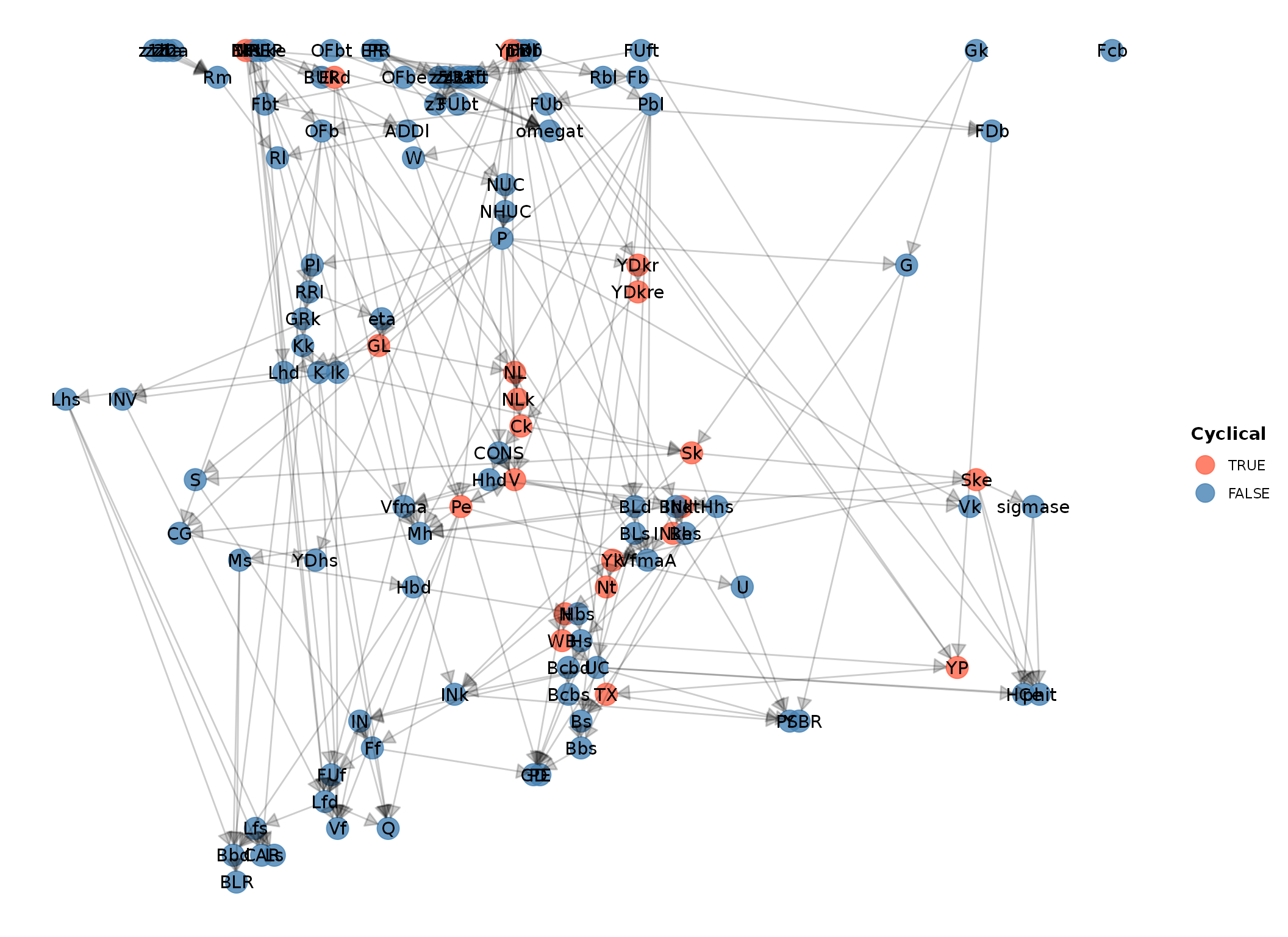

Structure of the model (DAG)

sfcr_dag_cycles_plot(growth_eqs, size = 6)

Scenario BENCHMARK: A continuation of baseline model

growthbl <- sfcr_scenario(
  baseline = growth,
  scenario = NULL,
  periods = 150,
  method = "Broyden"
)

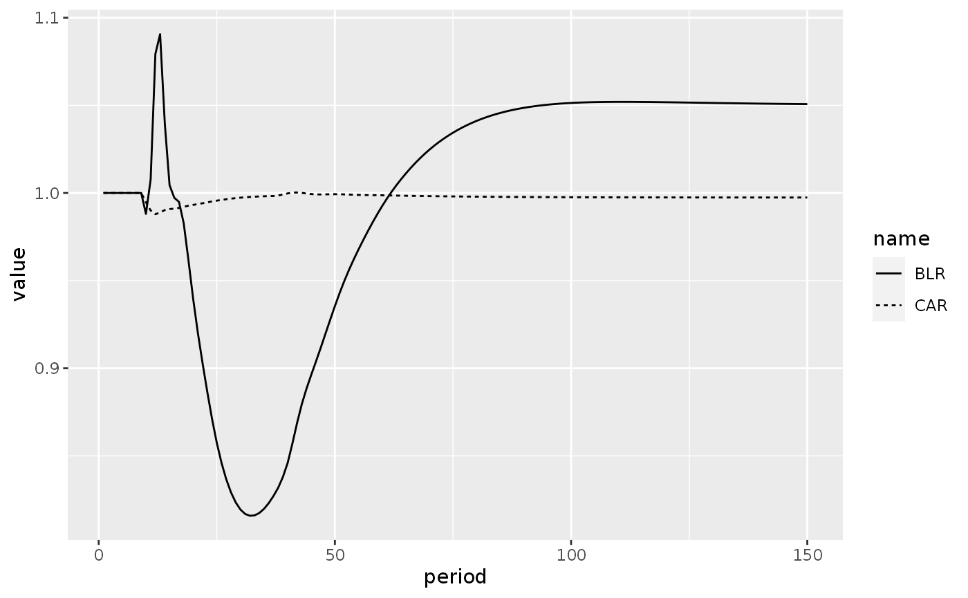
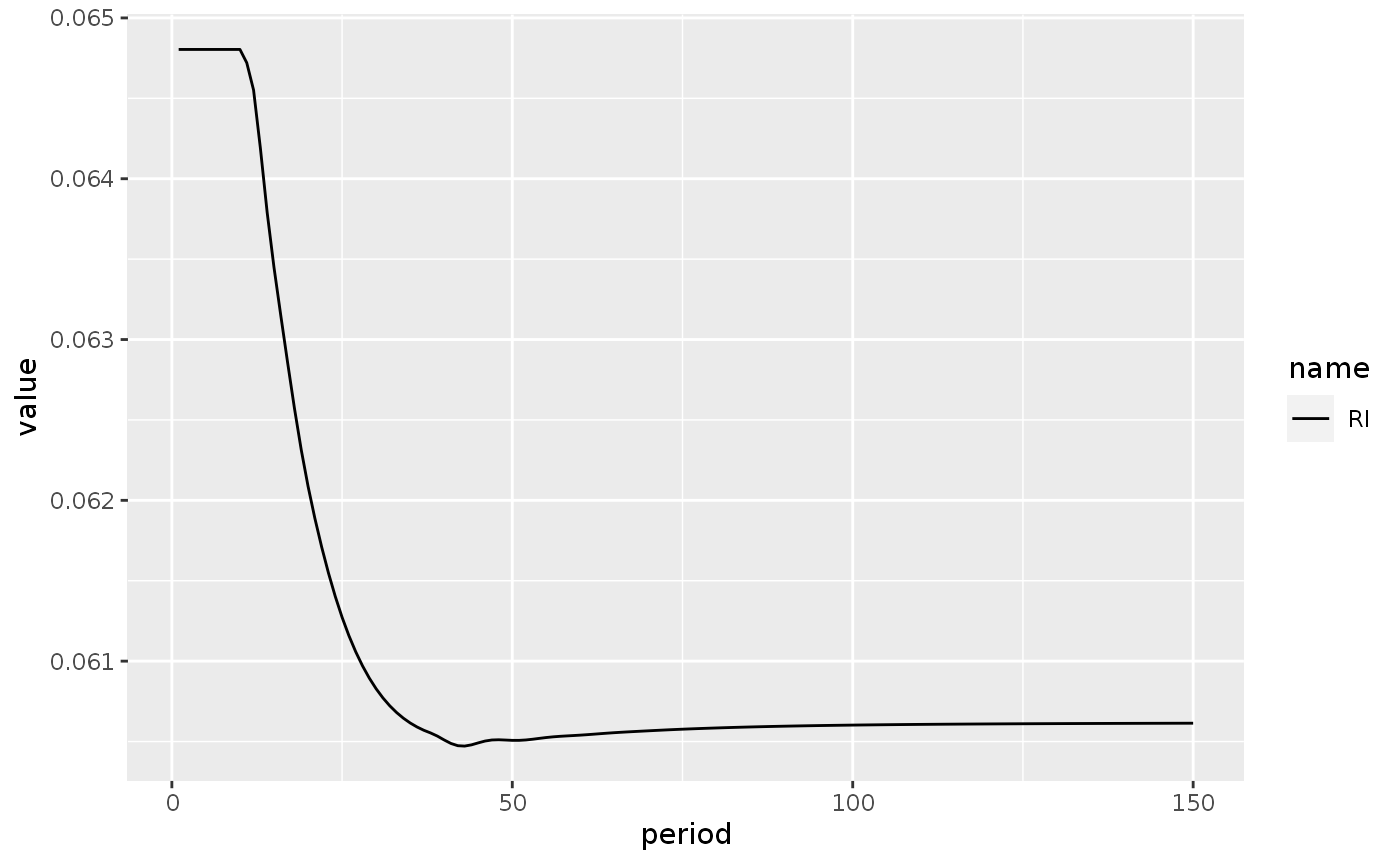
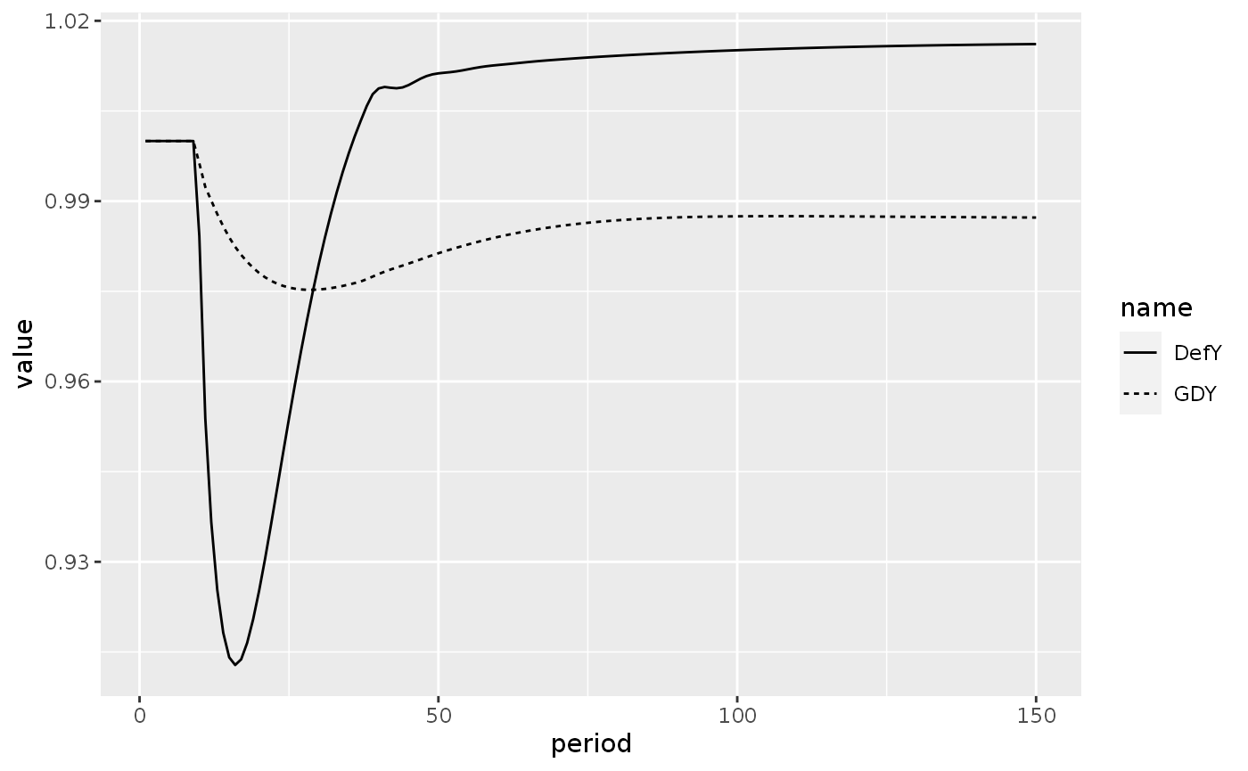
Scenario 1: Autonomous increase in the target real wage

shock1 <- sfcr_shock(
  variables = sfcr_set(
    omega0 ~ -0.1
  ),
  start = 5,
  end = 150
)

growtha <- sfcr_scenario(
  baseline = growth,
  scenario = shock1,
  periods = 150,
  method = "Broyden"
)

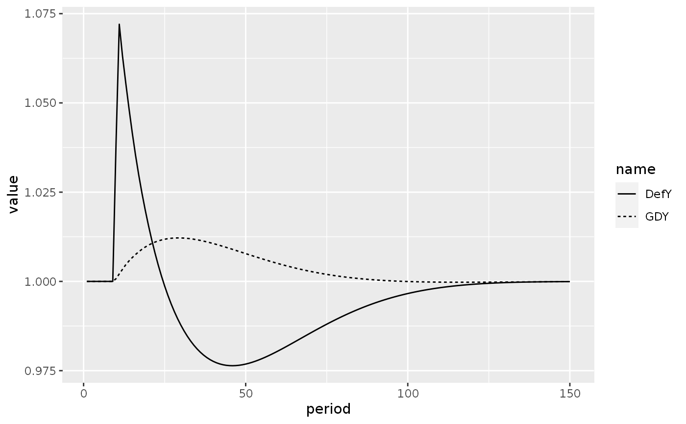
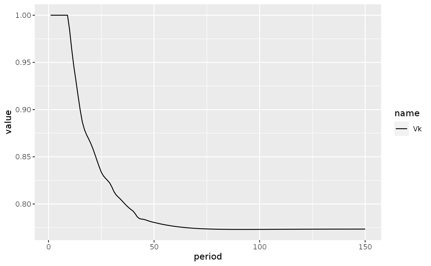
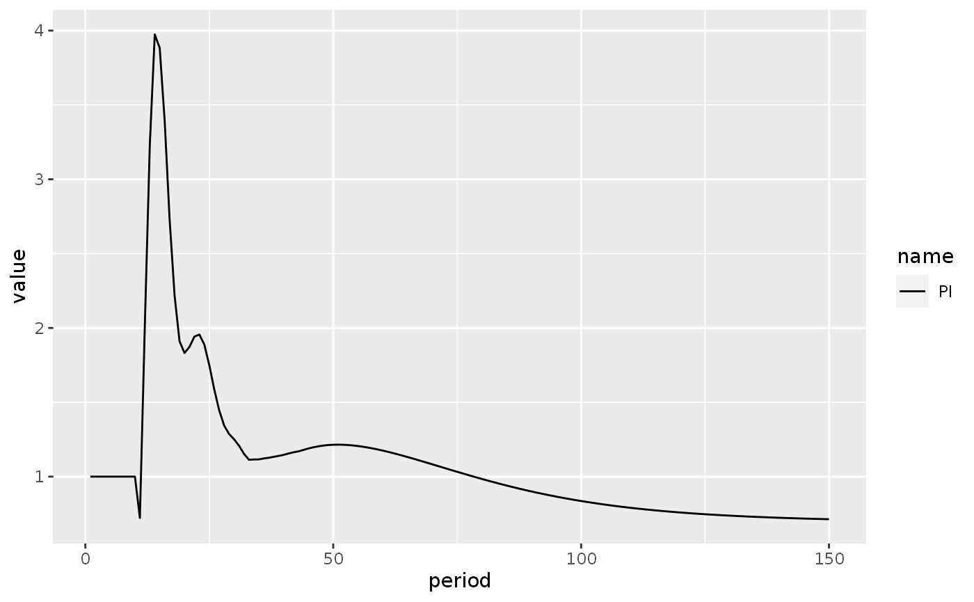
Figure 11.2A

growtha %>%
  do_plot(variables = c("PI", "wi")) +
  scale_y_continuous(labels = scales::percent)
#> Warning: Removed 1 row(s) containing missing values (geom_path).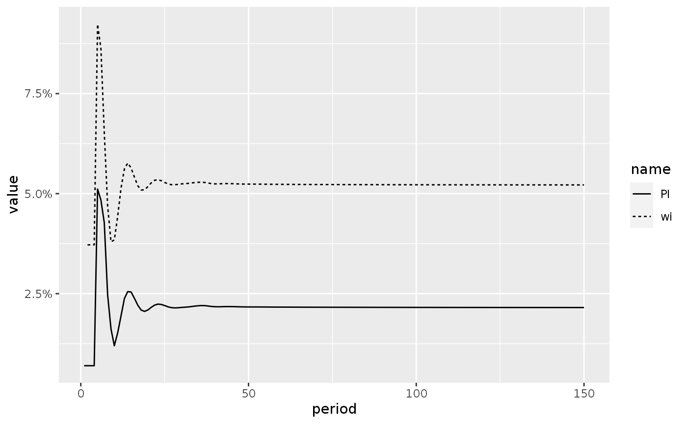

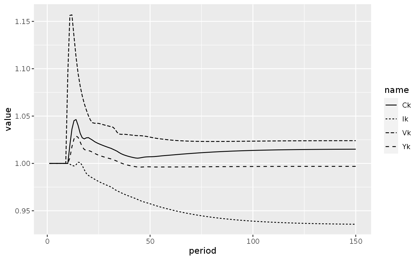
To generate the comparison of Figure 11.2A, we need to compare model growth1 against the counterfactual baseline evolution growthbl. The code below creates two helper functions that will divide the selected variables by their counterparts in the growthbl model and then apply the do_plot function to it.

do_cbind <- function(m1, m2, variables) {
  bind_cols(
    m1,
    select(m2, c(!!variables)) %>% set_names(paste0(names(.), "_bl"))
  )
}

do_cplot <- function(m1, variables, plot = NULL, m2 = growthbl) {
  vars = paste0(variables, "_bl")
  ntbl <- do_cbind(m1, m2, variables)
  for (.v in seq_along(variables)) {
    ntbl[, variables[[.v]]] <- ntbl[, variables[[.v]]] / ntbl[, vars[[.v]]]
  }
  ntbl %>%
    do_plot(variables, plot)
}

Figure 11.2B

do_cplot(growtha, c("Ik", "Ck", "Yk"))

Scenario 1, second experiment

shock2 <- sfcr_shock(
  variables = sfcr_set(
    Rbbar ~ 0.055
  ),
  start = 5,
  end = 150
)

growthab <- sfcr_scenario(
  baseline = growth,
  scenario = list(shock1, shock2),
  periods = 150,
  method = "Broyden"
)

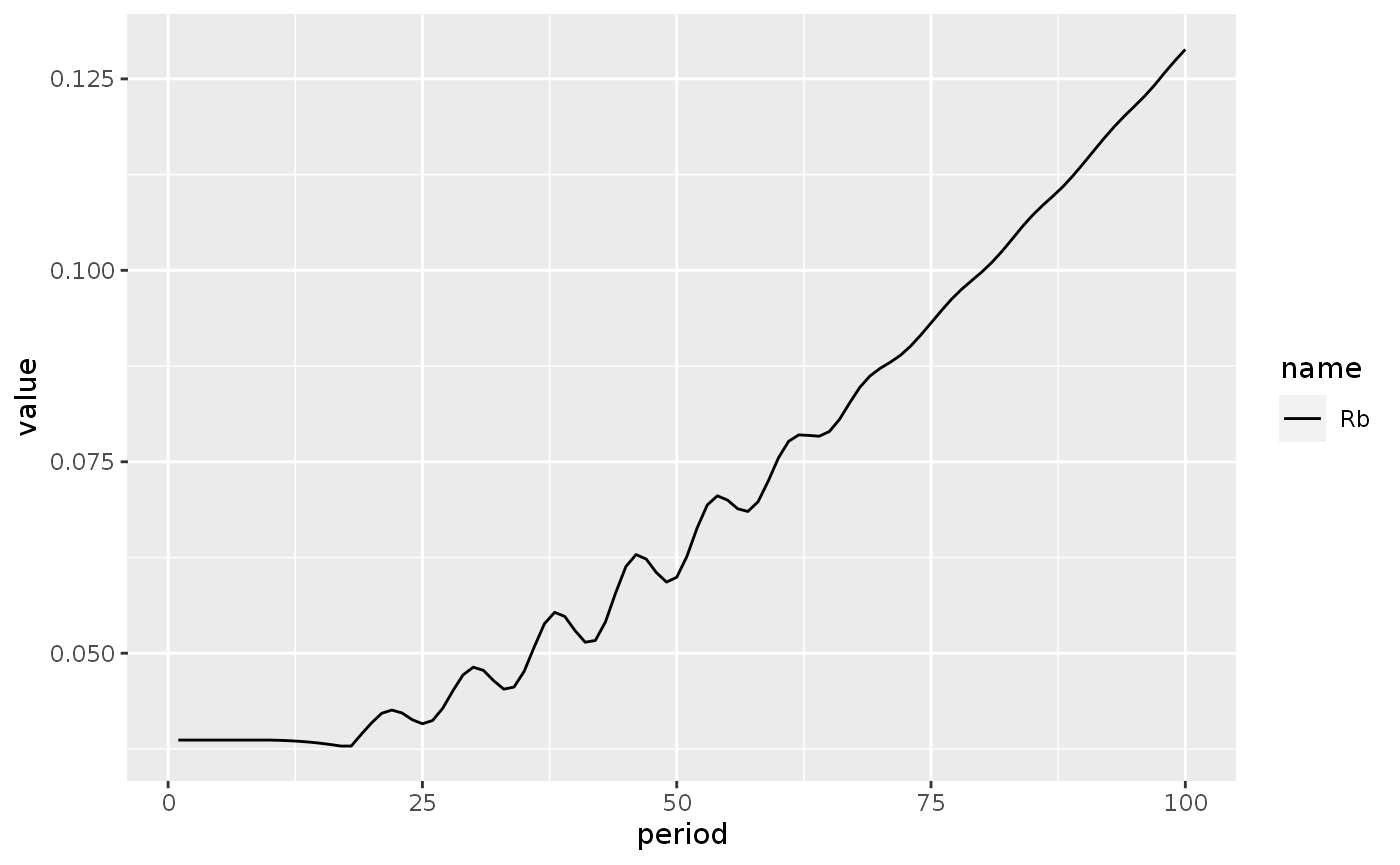
Figure 11.2C

This figure required some trial and error to find a value of Rbbar that makes the real interest on bills to end more or less where it started. Is there a way to automate this procedure?

Also note that the real interest rate in Godley and Lavoie (2007, 407) first increases and then it decreases. The only way to make something similar to that is to set the shock on interest rates to happens before the shock on inflation, which contradicts the book.

growthab %>%
  mutate(Rrb = Rb - PI) %>%
  do_plot(variables = "Rrb")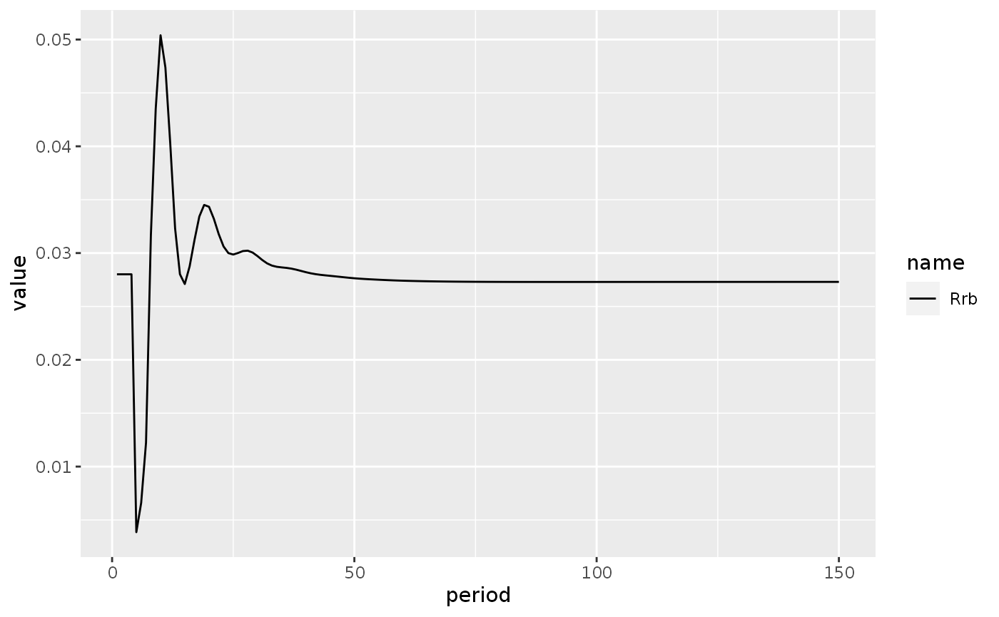

Figure 11.2D

do_cplot(growthab, variables = c("Yk"), plot = c("Yk"))

Scenario 2: One-period only increase in the growth rate of pure government expenditures

shock3 <- sfcr_shock(
  variables = sfcr_set(
    GRg ~ 0.035
  ),
  start = 10,
  end = 11
)

growthb <- sfcr_scenario(
  baseline = growth,
  scenario = shock3,
  periods = 150,
  method = "Broyden"
)

Figure 11.3A

do_cplot(growthb, variables = c("Yk", "Gk"), plot = c("Yk", "Gk"))

Figure 11.3B

do_cplot(growthb, c("ER")) +
  map(c(1.02, 0.98), ~geom_hline(yintercept = .x))

Figure 11.3C

do_cplot(growthb, variables = c("PSBR", "Y", "GD"), plot = c("DefY", "GDY"))

Figure 11.3D

do_cplot(growthb, variables = c("Lfd", "IN", "BLR"), plot = c("LIN", "BLR"))

Scenario 2.B: One-shot decrease in the income tax

shock4 <- sfcr_shock(
  variables = sfcr_set(
    theta ~ 0.22
  ),
  start = 10,
  end = 150
)

growthbb <- sfcr_scenario(
  baseline = growth,
  scenario = shock4,
  periods = 150,
  method = "Broyden"
)

Figure 11.3E

do_cplot(growthbb, v = c("Ck", "Yk"), p = c("Ck", "Yk"))

Scenario 3: A permanent increase in the growth rate of pure government expenditures

shock5 <- sfcr_shock(
  variables = sfcr_set(
    GRg ~ 0.035
  ),
  start = 10,
  end = 150
)

growthc <- sfcr_scenario(
  baseline = growth,
  scenario = shock5,
  periods = 150,
  method = "Broyden"
)

Figure 11.4A

do_plot(growthc, v = c("ER", "PI")) +
  facet_wrap(~name, scales = "free_y")

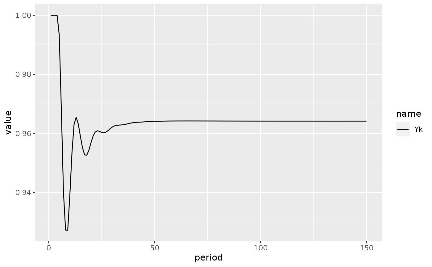
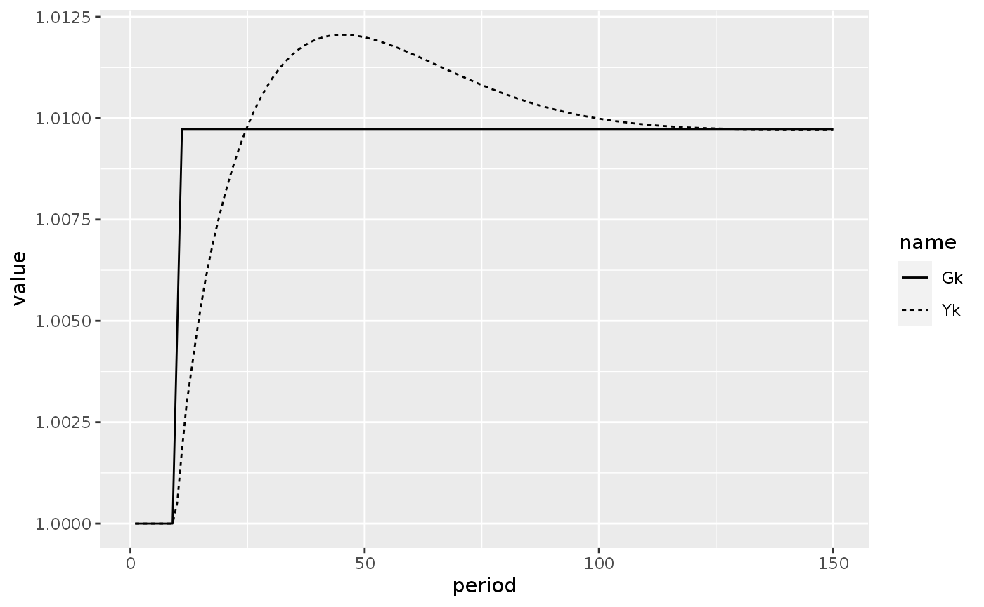
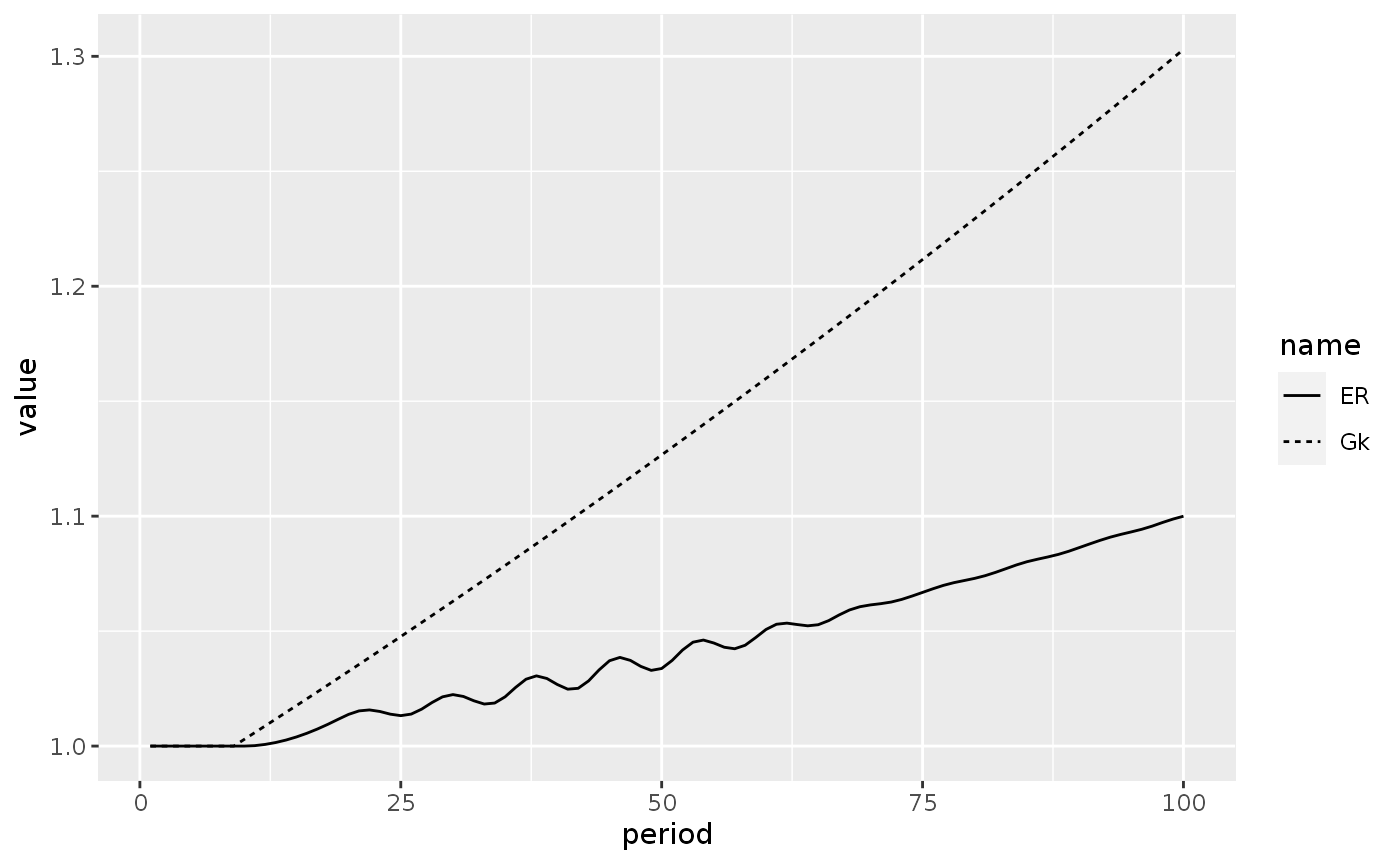
Figure 11.4B

do_plot(growthc, p = c("GRg", "GRk", "GRy"))
#> Warning: Removed 1 row(s) containing missing values (geom_path).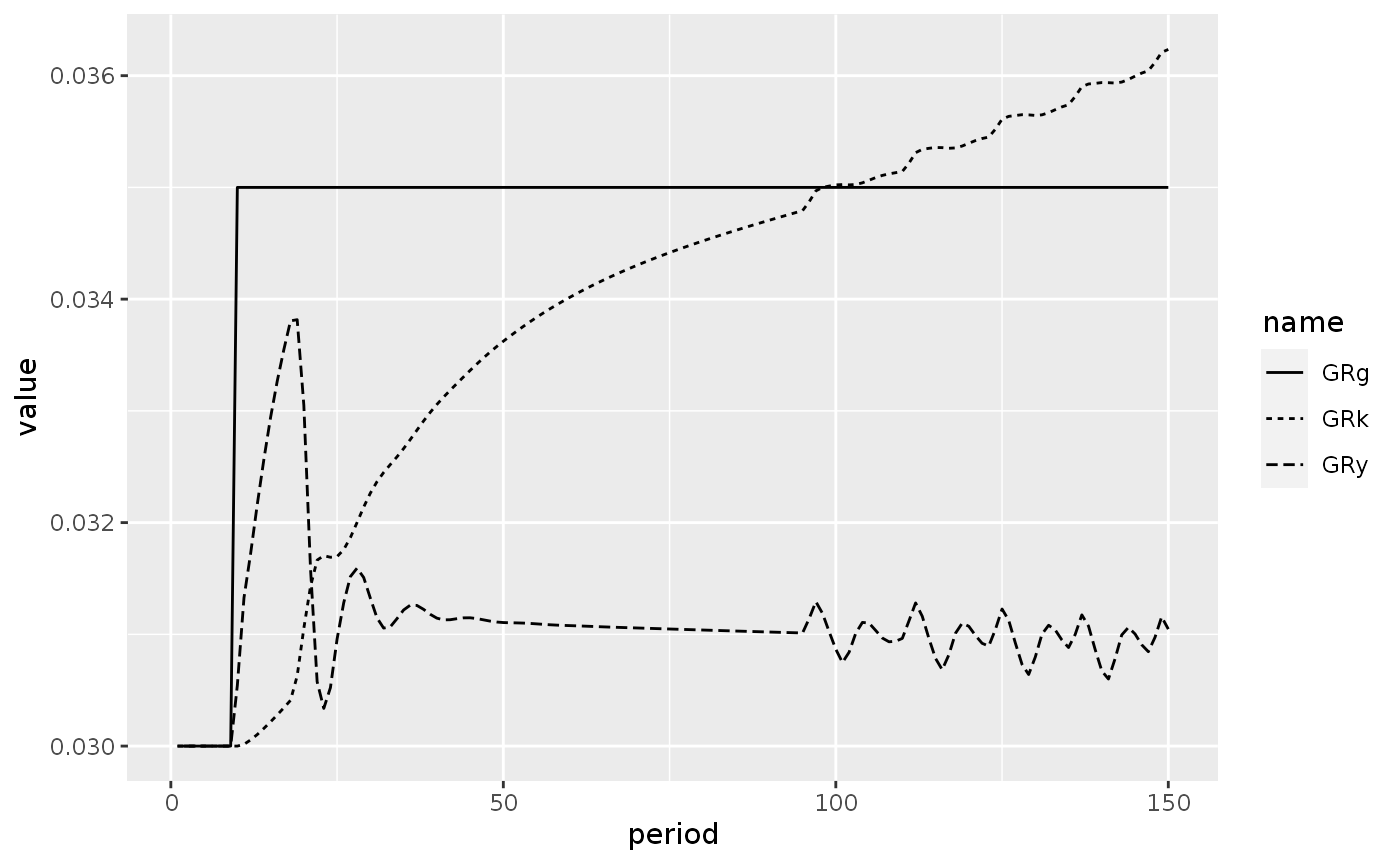

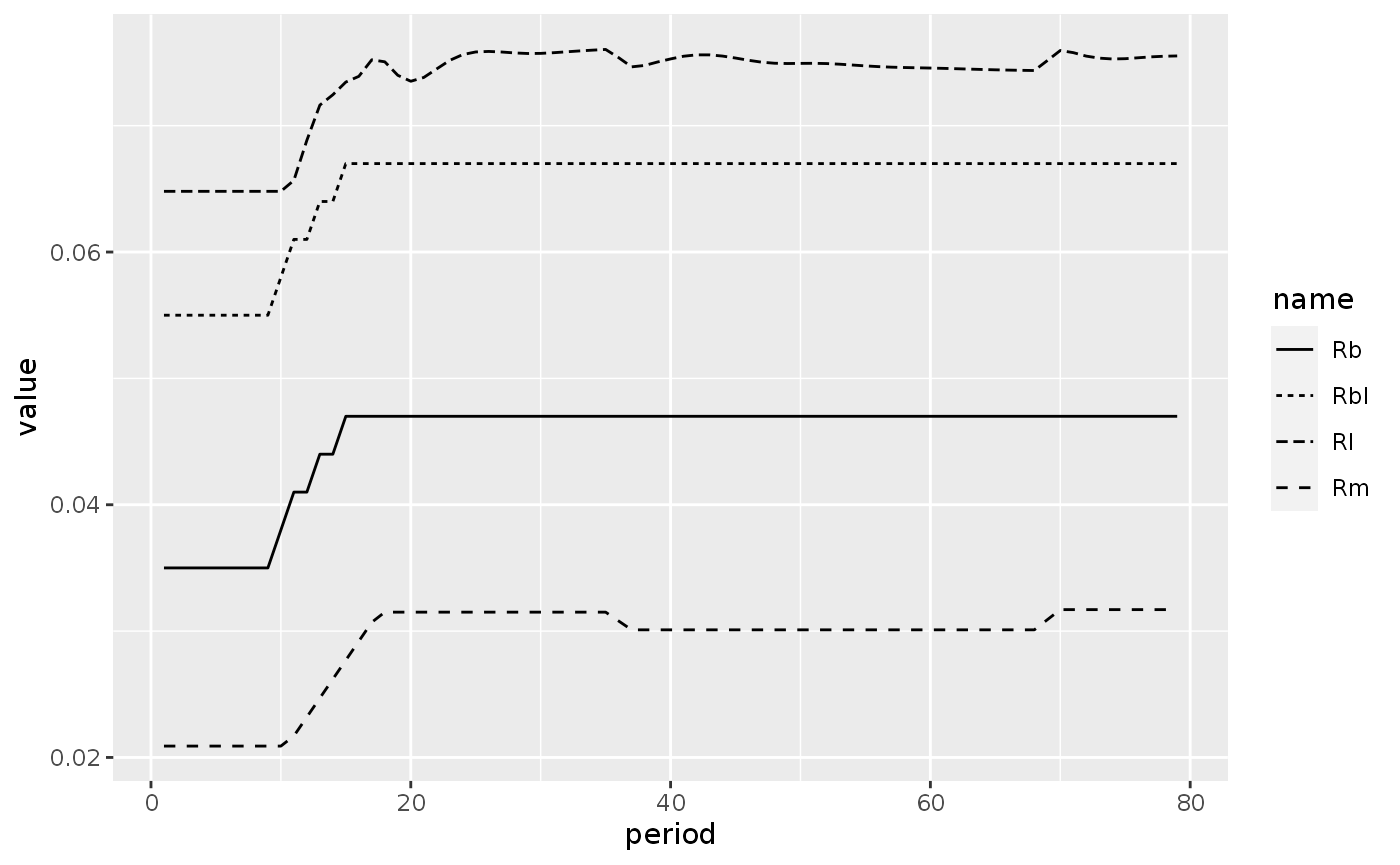
Figure 11.4C

do_plot(growthc, v = c("DefY", "GDY")) +
  facet_wrap(~name, scales = "free_y")

Scenario 4: A permanent increase in the bill rate of interest

shock6a <- sfcr_shock(v = sfcr_set(Rbbar ~ 0.038), s = 10, e = 11)
shock6b <- sfcr_shock(v = sfcr_set(Rbbar ~ 0.041), s = 11, e = 12)
shock6c <- sfcr_shock(v = sfcr_set(Rbbar ~ 0.044), s = 13, e = 14)
shock6d <- sfcr_shock(v = sfcr_set(Rbbar ~ 0.047), s = 15, e = 150)

growthd <- sfcr_scenario(
  baseline = growth,
  scenario = list(shock6a, shock6b, shock6c, shock6d),
  periods = 150,
  method = "Broyden"
)

Figure 11.5A

growthd %>%
  filter(period < 80) %>%
  do_plot(v = c("Rl", "Rbl", "Rb", "Rm"))

Figure 11.5B

do_cplot(growthd, v = c("Ck", "Yk"), p = c("Ck", "Yk"))

Figure 11.5C

do_cplot(growthd, v = c("GD", "Y"), p = "GDY")

Figure 11.5D

do_plot(growthd, v = c("LhYDr"))

Figure 11.5E

do_plot(growthd, v = c("BUR"))

Scenario 5: Increase in the propensity to consume out of regular income

shock7 <- sfcr_shock(v = sfcr_set(alpha1 ~ 0.80), s = 10, e = 150)

growthe <- sfcr_scenario(growth, shock7, 150, method = "Broyden")

Figure 11.7A

do_cplot(growthe, v = c("Ck", "Yk"), p = c("Ck", "Yk"))

Figure 11.7B

do_cplot(growthe, v = "Vk", p = "Vk")

Figure 11.7C

do_cplot(growthe, v = 'PI', p = "PI")

Figure 11.7D

do_cplot(growthe, v = c("NHUC", "phi"), p = c("NHUC", "phi"))

I invite the reader to make a smaller shock above and see what happens. Instead of making alpha1 equal to 0.80, make it equal to 0.77. This might come as a surprise…

Figure 11.7E

do_cplot(growthe, v = c("FUf", "INV", "INk"), p = c("FUfInv", "INk"))

Figure 11.7F

do_cplot(growthe, v = c("Y", "GD", "PSBR"), p = c("DefY", "GDY"))

Figure 11.7G

do_cplot(growthe, v = c("Q", 'PE'), p = c("Q", "PE"))

Scenario 7: An increase in the gross new loans to personal income ratio

shock8 <- sfcr_shock(v = sfcr_set(eta0 ~ 0.08416), s = 10, e = 150)
growthf <- sfcr_scenario(growth, shock8, 150, method = "Broyden")

Figure 11.8A

growthf %>%
  do_plot(v = c("LhYDr", "BUR")) +
  facet_wrap(~name, scales = "free_y")

Figure 11.8B

do_cplot(growthf, v = c("Yk", "Ck"), p = c("Yk", "Ck"))

Figure 11.8C

do_cplot(growthf, v = c("BLR", "CAR"), p = c("BLR", "CAR"))

Figure 11.8D

do_plot(growthf, "Rl")

Figure 11.8E

do_cplot(growthf, v = c("Y", "PSBR", "GD"), p = c("DefY", "GDY"))

Scenario 8: An increase in the desire to hold equities

This scenario changes one of the portfolio parameters. We can change only one parameter without affecting the consistency of the model since such changes are counterbalanced by changes in the hidden deposit parameters (that are not explicitly modelled).

shock9 <- sfcr_shock(v = sfcr_set(lambda40 ~ 0.77132), s = 10, e = 150)
growthg <- sfcr_scenario(growth, shock9, 150, method = "Broyden")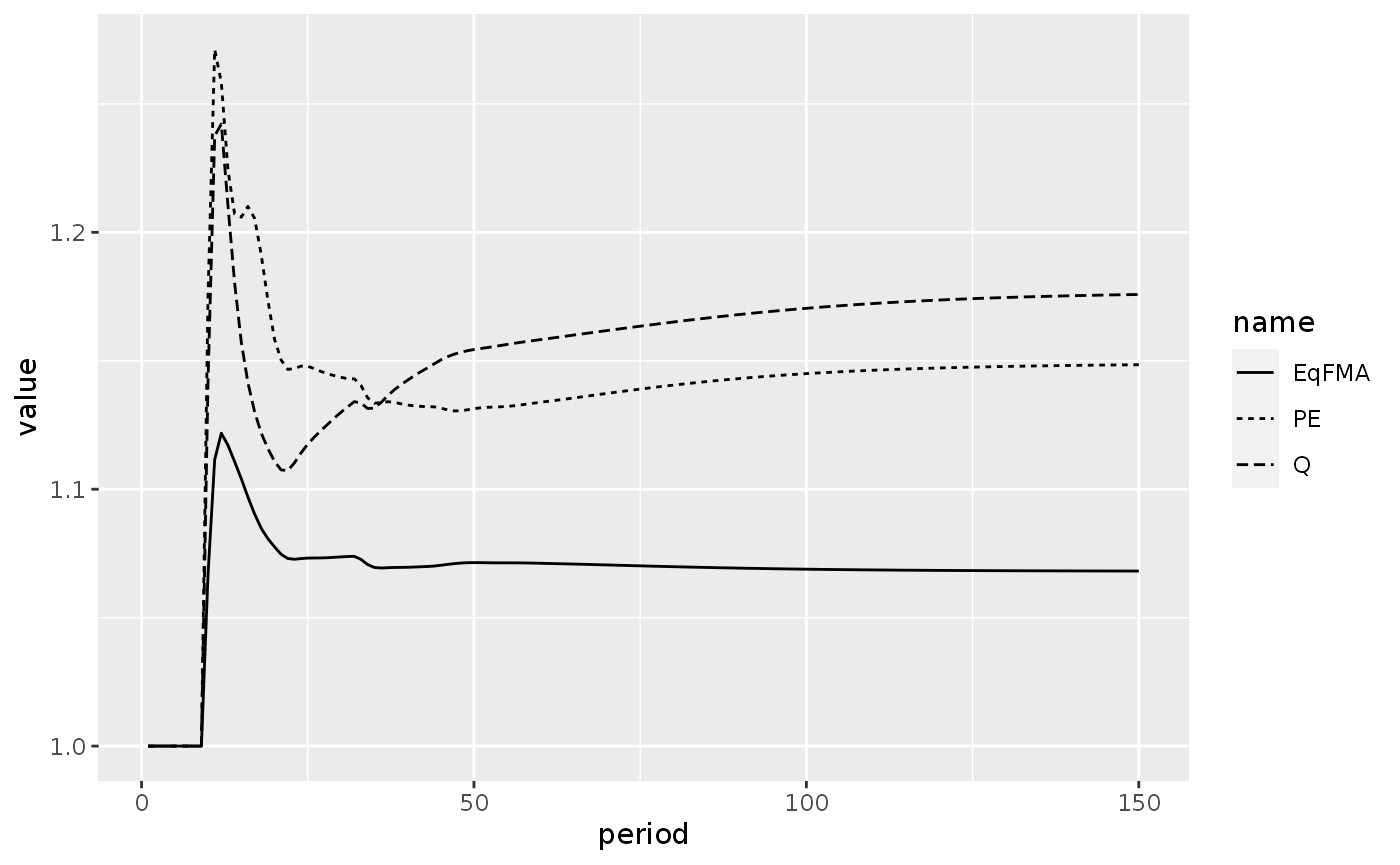

Figure 11.9A

do_cplot(growthg, v = c("Q", "PE", "Ekd", "Pe", "Vfma"), p = c("Q", "PE", "EqFMA"))

Figure 11.9B

do_cplot(growthg, v = c("Ck", "Vk", "Yk", "Ik"), p = c("Ck", "Vk", "Yk", "Ik"))

Figure 11.9C

do_plot(growthg, v = c("Rl", "Rm"))

Scenario 8b: Increase in the desire to hold equities that is offset by a decline in the desire to hold bills and bonds

shock10 <- sfcr_shock(
  v = sfcr_set(
    lambda20 ~ 0.20,
    lambda30 ~ -0.09341),
  s = 10,
  e = 150)

growthgb <- sfcr_scenario(growth, list(shock9, shock10), 150, method = "Broyden")

Figure 11.9D

growthgb %>%
  do_plot(v = c("Rl", "Rb", "Rm"))

Scenario 9: An increase in the target proportion of gross investment financed by retained earnings

shock11 <- sfcr_shock(v = sfcr_set(psiu ~ 1), s = 10, e = 150)
growthh <- sfcr_scenario(growth, shock11, 150, method = "Broyden")

Figure 11.10A

do_plot(growthh, "phi")

Figure 11.10B

growthh %>% do_plot("wi")
#> Warning: Removed 1 row(s) containing missing values (geom_path).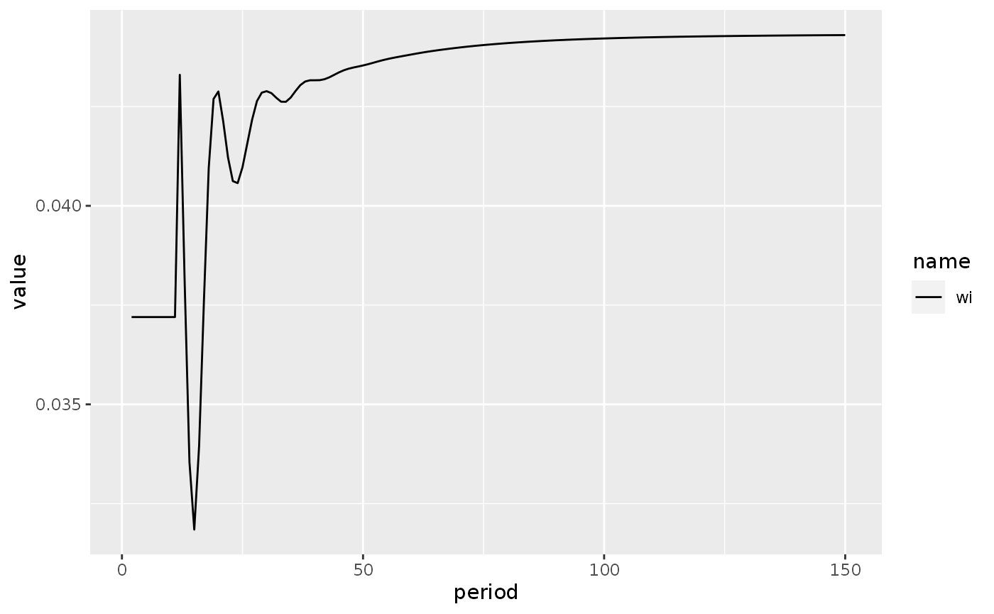

Figure 11.10C

do_cplot(growthh, v = c("ER", "Ck"), p = c("ER", "Ck"))

Figure 11.10D

do_cplot(growthh, v = c("Q", "PE"), p = c("Q", "PE"))

Figure 11.10E

do_plot(growthh, v = c("GRFfk", "GRPek"))
#> Warning: Removed 2 row(s) containing missing values (geom_path).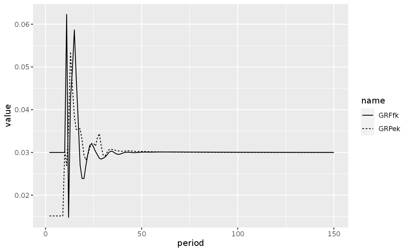

Scenario 10: An increase in non-performing loans

shock12 <- sfcr_shock(v = sfcr_set(NPLk ~ 0.05), s = 10, e = 150)
growthi <- sfcr_scenario(growth, shock12, 150, method = "Broyden")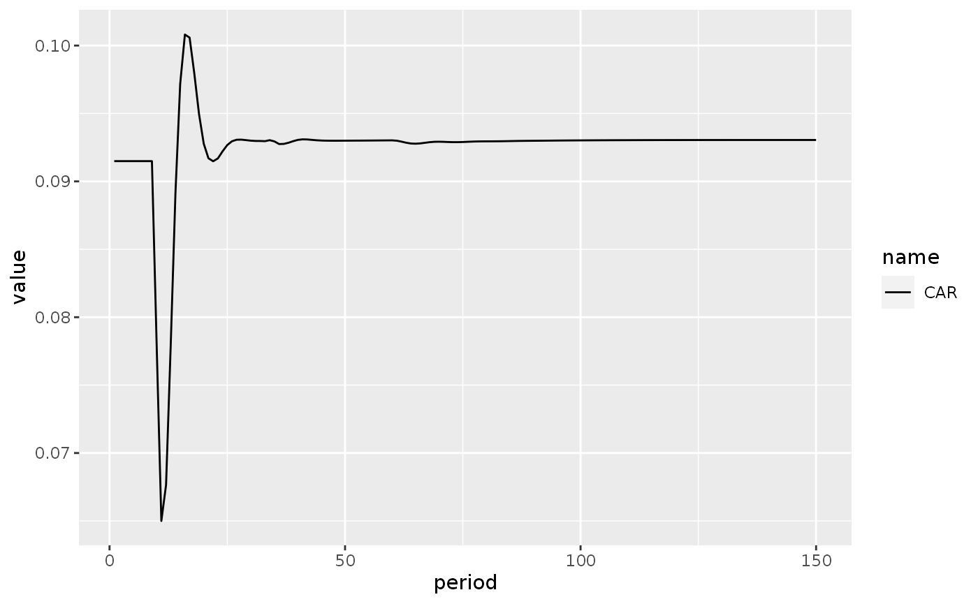

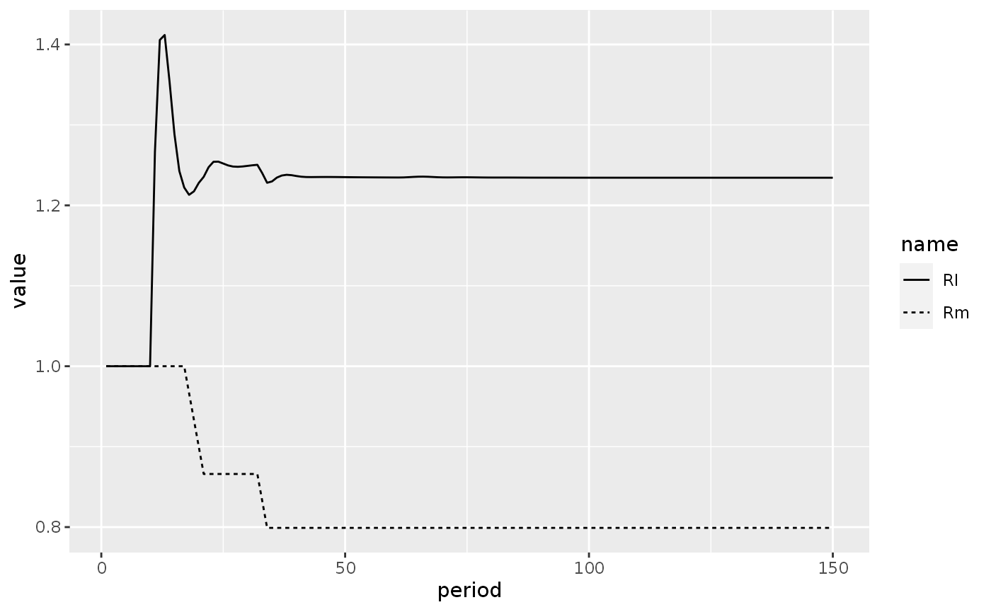
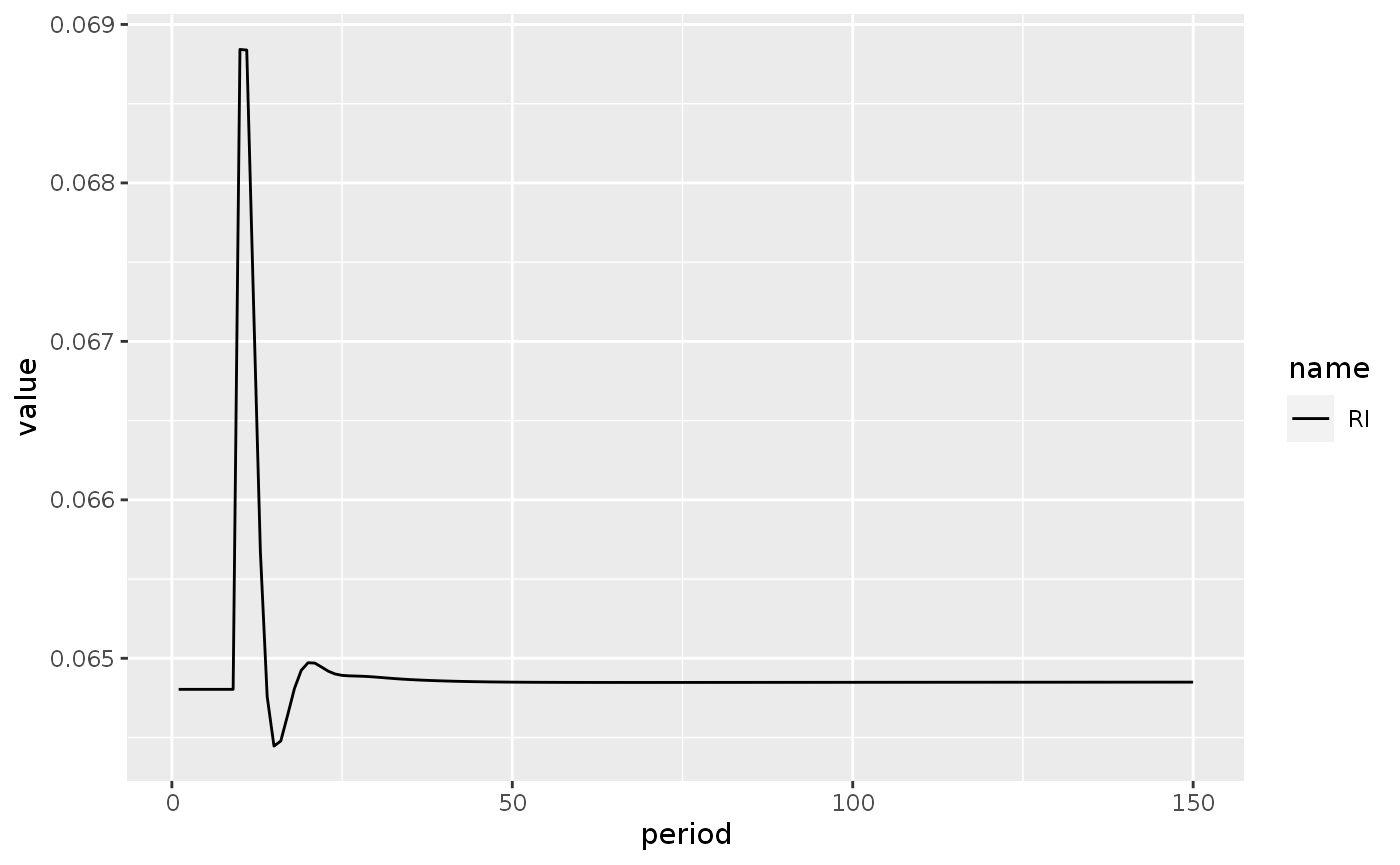
Figure 11.11A

do_plot(growthi, "CAR")

Figure 11.11B

do_cplot(growthi, v = c("Rm", "Rl"), p = c("Rm", "Rl"))

Scenario 10B: An increase in the normal adequacy ratio

shock13 <- sfcr_shock(v = sfcr_set(NCAR ~ 0.11), s = 10, e = 150)
growthib <- sfcr_scenario(growth, shock13, 150, method = "Broyden")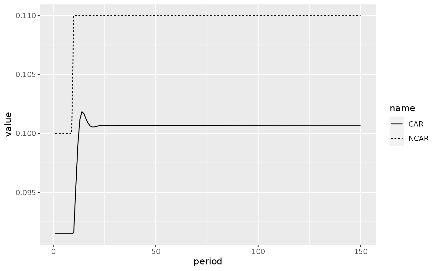

Figure 11.11C

do_plot(growthib, v = c("NCAR", "CAR"))

Figure 11.11D

do_plot(growthib, "Rl")

Model GROWTH2: Making monetary policy endogenous

growth_eqs2 <- growth_eqs
growth_eqs2[[88]] <- Rb ~  (1 + Rrb) * (1 + PI) - 1
growth_eqs2 <- c(
  growth_eqs2,
  Rrbt ~  (1 + Rb)/(1 + PI) - 1,
  Rrb ~ Rrb[-1] + epsrb * (Rrbt - Rrb[-1])
)

growth_parameters2 <- c(
  growth_parameters,
  epsrb ~ 0.9
)

growth_initial2 <- c(
  growth_initial,
  Rrbt ~ 0.03232,
  epsrb ~ 0.9,
  Rrb ~  0.03232
)

growth2 <- sfcr_baseline(
  equations = growth_eqs2,
  external = growth_parameters2,
  periods = 350,
  initial = growth_initial2,
  hidden = c("Bbs" = "Bbd"),
  .hidden_tol = 1e-6,
  method = "Broyden",
  rhtol = TRUE
)

Steady state

We can see that this model arrives to a steady state:

growth2 %>%
  do_plot(variables = c("Uk", "Bsk", "VK", 'GRk', "PI")) +
    facet_wrap(~name, scales = "free_y")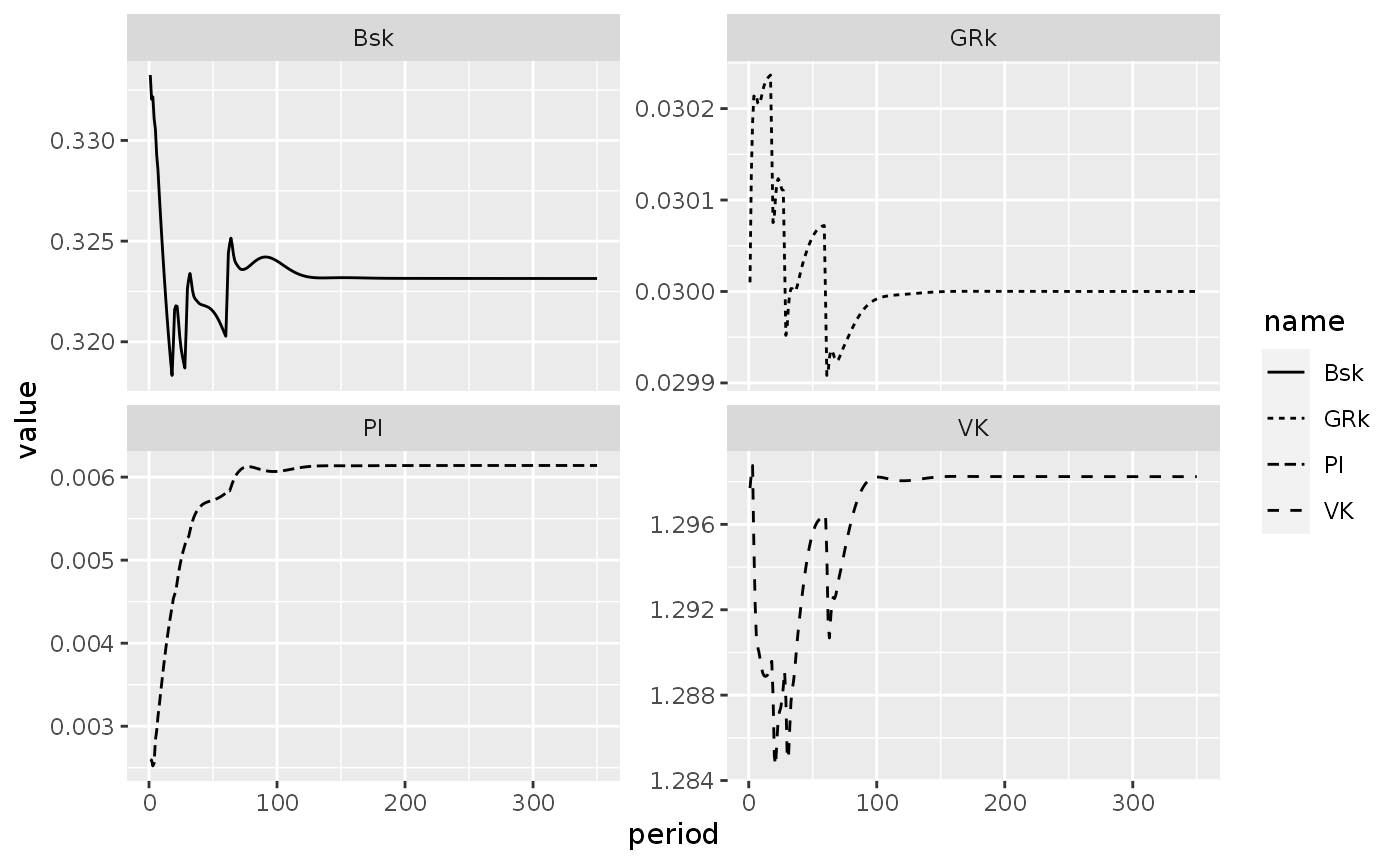

Scenario benchmark

growthbl2 <- sfcr_scenario(
  growth2,
  NULL,
  100,
  method = "Broyden"
)

Scenario 1: Permanent increase in government expenditures

This model is rather unstable and breaks the Broyden/Gauss algorithms if run for many periods (I couldn’t make it run with 150 periods). Sometimes it did run with Newton method and sometimes it didn’t.

shock1 <- sfcr_shock(v = sfcr_set(GRg ~ 0.033), s = 10, e = 100)

growth2a <- sfcr_scenario(
  baseline = growth2,
  scenario = shock1,
  periods = 100,
  method = "Broyden"
)

Figure 11.6A

do_plot(growth2a, c("GRy"))
#> Warning: Removed 1 row(s) containing missing values (geom_path).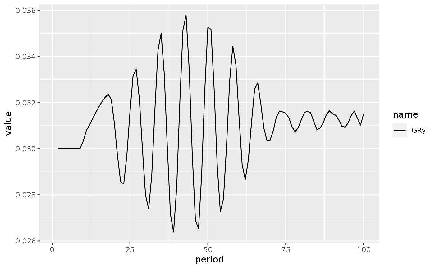

Figure 11.6B

do_plot(growth2a, c("Rb"))

Figure 11.6C

growth2a %>%
  do_cplot(v = c("Gk", "ER"), p = c("Gk", "ER"), m2 = growthbl2)

Figure 11.6D

growth2a %>%
  do_plot(v = c("Rl", "Rb", "Rm"))

Session information

sessionInfo()
#> R version 4.0.2 (2020-06-22)
#> Platform: x86_64-pc-linux-gnu (64-bit)
#> Running under: Ubuntu 16.04.6 LTS
#> 
#> Matrix products: default
#> BLAS:   /usr/lib/openblas-base/libblas.so.3
#> LAPACK: /usr/lib/libopenblasp-r0.2.18.so
#> 
#> locale:
#>  [1] LC_CTYPE=en_US.UTF-8       LC_NUMERIC=C              
#>  [3] LC_TIME=en_US.UTF-8        LC_COLLATE=en_US.UTF-8    
#>  [5] LC_MONETARY=en_US.UTF-8    LC_MESSAGES=en_US.UTF-8   
#>  [7] LC_PAPER=en_US.UTF-8       LC_NAME=C                 
#>  [9] LC_ADDRESS=C               LC_TELEPHONE=C            
#> [11] LC_MEASUREMENT=en_US.UTF-8 LC_IDENTIFICATION=C       
#> 
#> attached base packages:
#> [1] stats     graphics  grDevices utils     datasets  methods   base     
#> 
#> other attached packages:
#>  [1] forcats_0.5.1   stringr_1.4.0   dplyr_1.0.7     purrr_0.3.4    
#>  [5] readr_2.0.2     tidyr_1.1.4     tibble_3.1.5    ggplot2_3.3.5  
#>  [9] tidyverse_1.3.1 sfcr_0.2.1     
#> 
#> loaded via a namespace (and not attached):
#>  [1] fs_1.5.0           lubridate_1.8.0    webshot_0.5.2      httr_1.4.2        
#>  [5] rprojroot_2.0.2    tools_4.0.2        backports_1.2.1    utf8_1.2.2        
#>  [9] R6_2.5.1           DBI_1.1.1          colorspace_2.0-2   withr_2.4.2       
#> [13] gridExtra_2.3      tidyselect_1.1.1   compiler_4.0.2     textshaping_0.3.5 
#> [17] cli_3.0.1          rvest_1.0.1        expm_0.999-6       xml2_1.3.2        
#> [21] desc_1.4.0         labeling_0.4.2     scales_1.1.1       pkgdown_1.6.1     
#> [25] systemfonts_1.0.2  digest_0.6.28      rmarkdown_2.11     svglite_2.0.0     
#> [29] pkgconfig_2.0.3    htmltools_0.5.2    dbplyr_2.1.1       fastmap_1.1.0     
#> [33] highr_0.9          htmlwidgets_1.5.4  rlang_0.4.11       readxl_1.3.1      
#> [37] rstudioapi_0.13    jquerylib_0.1.4    farver_2.1.0       generics_0.1.0    
#> [41] jsonlite_1.7.2     magrittr_2.0.1     kableExtra_1.3.4   Matrix_1.2-18     
#> [45] Rcpp_1.0.7         munsell_0.5.0      fansi_0.5.0        viridis_0.6.1     
#> [49] lifecycle_1.0.1    stringi_1.7.5      yaml_2.2.1         ggraph_2.0.5      
#> [53] MASS_7.3-51.6      rootSolve_1.8.2.3  grid_4.0.2         ggrepel_0.9.1     
#> [57] crayon_1.4.1       lattice_0.20-41    graphlayouts_0.7.1 haven_2.4.3       
#> [61] hms_1.1.1          knitr_1.36         pillar_1.6.3       igraph_1.2.6      
#> [65] reprex_2.0.1       glue_1.4.2         evaluate_0.14      modelr_0.1.8      
#> [69] tweenr_1.0.2       vctrs_0.3.8        tzdb_0.1.2         Rdpack_2.1.2      
#> [73] networkD3_0.4      cellranger_1.1.0   polyclip_1.10-0    gtable_0.3.0      
#> [77] assertthat_0.2.1   cachem_1.0.6       ggforce_0.3.3      xfun_0.26         
#> [81] rbibutils_2.2.4    broom_0.7.9        tidygraph_1.2.0    ragg_1.1.3        
#> [85] viridisLite_0.4.0  memoise_2.0.0      ellipsis_0.3.2

References

Godley, Wynne, and Marc Lavoie. 2007. Monetary Economics: An Integrated Approach to Credit, Money, Income, Production and Wealth. Palgrave Macmillan.

Chapter 11: Model GROWTH

Equations, parameters, and initial values

Model GROWTH: Baseline

The hidden equation: is it fulfilled?

Steady state

Matrices of model GROWTH

Balance-sheet matrix

Transactions-flow matrix

Sankey’s diagram:

Structure of the model (DAG)

Scenario BENCHMARK: A continuation of baseline model

Scenario 1: Autonomous increase in the target real wage

Figure 11.2A

Figure 11.2B

Scenario 1, second experiment

Figure 11.2C

Figure 11.2D

Scenario 2: One-period only increase in the growth rate of pure government expenditures

Figure 11.3A

Figure 11.3B

Figure 11.3C

Figure 11.3D

Scenario 2.B: One-shot decrease in the income tax

Figure 11.3E

Scenario 3: A permanent increase in the growth rate of pure government expenditures

Figure 11.4A

Figure 11.4B

Figure 11.4C

Scenario 4: A permanent increase in the bill rate of interest

Figure 11.5A

Figure 11.5B

Figure 11.5C

Figure 11.5D

Figure 11.5E

Scenario 5: Increase in the propensity to consume out of regular income

Figure 11.7A

Figure 11.7B

Figure 11.7C

Figure 11.7D

Figure 11.7E

Figure 11.7F

Figure 11.7G

Scenario 7: An increase in the gross new loans to personal income ratio

Figure 11.8A

Figure 11.8B

Figure 11.8C

Figure 11.8D

Figure 11.8E

Scenario 8: An increase in the desire to hold equities

Figure 11.9A

Figure 11.9B

Figure 11.9C

Scenario 8b: Increase in the desire to hold equities that is offset by a decline in the desire to hold bills and bonds

Figure 11.9D

Scenario 9: An increase in the target proportion of gross investment financed by retained earnings

Figure 11.10A

Figure 11.10B

Figure 11.10C

Figure 11.10D

Figure 11.10E

Scenario 10: An increase in non-performing loans

Figure 11.11A

Figure 11.11B

Scenario 10B: An increase in the normal adequacy ratio

Figure 11.11C

Figure 11.11D

Model GROWTH2: Making monetary policy endogenous

Steady state

Scenario benchmark

Scenario 1: Permanent increase in government expenditures

Figure 11.6A

Figure 11.6B

Figure 11.6C

Figure 11.6D

Session information

References