Load the required packages for this analysis:
library(sfcr)
library(tidyverse)
#> ── Attaching packages ─────────────────────────────────────── tidyverse 1.3.1 ──
#> ✔ ggplot2 3.3.5     ✔ purrr   0.3.4
#> ✔ tibble  3.1.5     ✔ dplyr   1.0.7
#> ✔ tidyr   1.1.4     ✔ stringr 1.4.0
#> ✔ readr   2.0.2     ✔ forcats 0.5.1
#> ── Conflicts ────────────────────────────────────────── tidyverse_conflicts() ──
#> ✖ dplyr::filter() masks stats::filter()
#> ✖ dplyr::lag()    masks stats::lag()
Bank-Money World model
Equations
- Write down the equations of the model:
bmw_eqs <- sfcr_set(
  # Basic behavioral equations
  Cs ~ Cd,
  Is ~ Id,
  Ns ~ Nd,
  Ls ~ Ls[-1] + Ld - Ld[-1],

  # Transactions of the firms
  Y ~ Cs + Is,
  WBd ~ Y - rl[-1] * Ld[-1] - AF,
  AF ~ delta * K[-1],
  Ld ~ Ld[-1] + Id - AF,

  # Transactions of households
  YD ~ WBs + rm[-1] * Mh[-1],
  Mh ~ Mh[-1] + YD - Cd,

  # Transactions of the banks
  Ms ~ Ms[-1] + Ls - Ls[-1],
  rm ~ rl,

  # The wage bill
  WBs ~ W * Ns,
  Nd ~ Y / pr,
  W ~ WBd / Nd,

  # Household behavior
  Cd ~ alpha0 + alpha1 * YD + alpha2 * Mh[-1],

  # The investment behavior
  K ~ K[-1] + Id - DA,
  DA ~ delta * K[-1],
  KT ~ kappa * Y[-1],
  Id ~ gamma * (KT - K[-1]) + DA
)

bmw_external <- sfcr_set(
  rl ~ 0.025,
  alpha0 ~ 20,
  alpha1 ~ 0.75,
  alpha2 ~ 0.10,
  delta ~ 0.10,
  gamma ~ 0.15,
  kappa ~ 1,
  pr ~ 1
)
Baseline
This model is tricky. The “Broyden” does not converge to a sensible answer if we don’t set the initial values of the following variables to reasonably large values (as the ones below). Interestingly, the other two solvers (“Gauss” and “Newton”) succeed in arriving to a sensible steady state without setting the initial values:
bmw_initial <- sfcr_set(
    Ns ~ 128, # Needs to be set
    Ls ~ 12, # Needs to be set
    Y ~ 128, # Needs to be set
    Ld ~ 12, # Needs to be set
    Mh ~ 12, # Needs to be set
    Ms ~ 12, # Needs to be set
    Nd ~ 128, # Needs to be set
    )

bmw <- sfcr_baseline(bmw_eqs, bmw_external, periods = 100, initial = bmw_initial, method = "Broyden", hidden = c("Ms" = "Mh"))
bmw <- sfcr_baseline(bmw_eqs, bmw_external, periods = 100, method = "Newton", hidden = c("Ms" = "Mh"))DAG
Let’s check the internal structure of this model with the sfcr_dag_blocks_plot() function:
sfcr_dag_blocks_plot(bmw_eqs)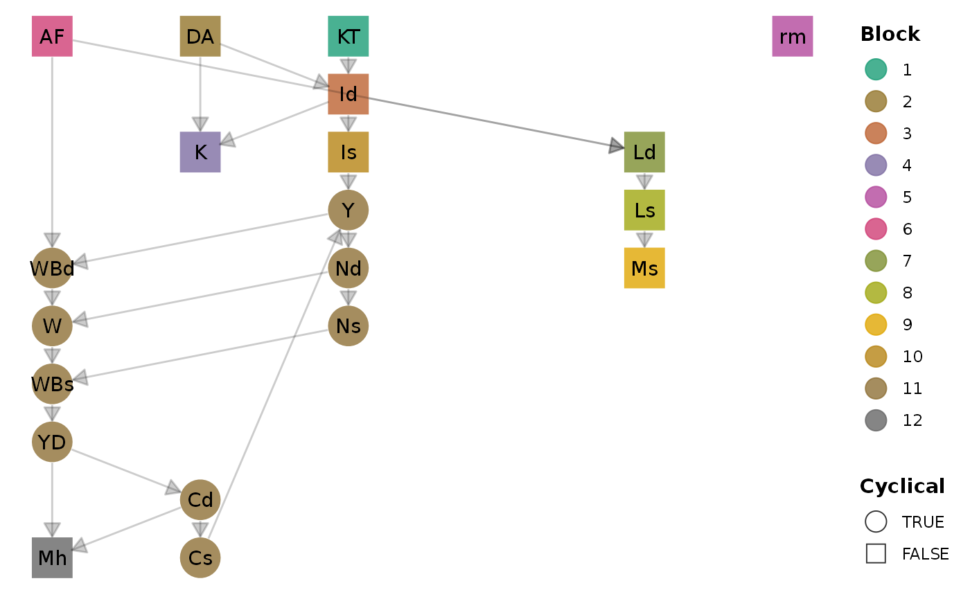
First, let’s check that the model arrived to a steady state income level:
bmw %>%
  pivot_longer(cols = -period) %>%
  filter(name == "Y") %>%
  ggplot(aes(x = period, y = value)) +
  geom_line() +
  labs(title = "Steady state GDP")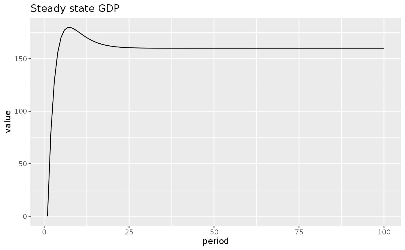
Matrices of model BMW
Balance-sheet
bs_bmw <- sfcr_matrix(
  columns = c("Households", "Firms", "Banks", "Sum"),
  codes = c("h", "f", "b", "s"),
  c("Money", h = "+Mh", b = "-Ms"),
  c("Loans", f = "-Ld", b = "+Ls"),
  c("Fixed capital", f = "+K", s = "+K"),
  c("Balance", h = "-Mh", s = "-Mh")
)
Validate:
sfcr_validate(bs_bmw, bmw, "bs")
#> Water tight! The balance-sheet matrix is consistent with the simulated model.
Transactions-flow
tfm_bmw <- sfcr_matrix(
  columns = c("Households", "Firms_current", "Firms_capital", "Banks_current", "Banks_capital"),
  codes = c("h", "fc", "fk", "bc", "bk"),
  c("Consumption", h ="-Cs", fc = "+Cd"),
  c("Investment", fc = "+Is", fk = "-Id"),
  c("Wages", h = "+WBs", fc = "-WBd"),
  c("Depreciation", fc = "-AF", fk = "+AF"),
  c("Interest loans", fc = "-rl[-1] * Ld[-1]", bc = "+rl[-1] * Ls[-1]"),
  c("Interest on deposits", h = "+rm[-1] * Mh[-1]", bc = "-rm[-1] * Ms[-1]"),
  c("Ch. loans", fk = "+d(Ld)", bk = "-d(Ls)"),
  c("Ch. deposits", h = "-d(Mh)", bk = "+d(Ms)")
)
sfcr_validate(tfm_bmw, bmw, "tfm")
#> Water tight! The transactions-flow matrix is consistent with the simulated model.
Now we add some shocks to this model to see how it behaves in different scenarios.
Scenario 1: An increase in autonomous consumption expenditures
First, let’s write a helper function to convert the models to the long format, filter the variables we want to plot, and make a line plot:
do_plot <- function(model, variables, title = NULL) {
  model %>%
    mutate(YK = Y / lag(K)) %>%
    pivot_longer(cols = -period) %>%
    filter(name %in% variables) %>%
    ggplot(aes(x = period, y = value)) +
    geom_line(aes(linetype = name)) +
    labs(title = title)
}
We then write the shock we want to add and simulate the new scenario:
shock1 <- sfcr_shock(
  variables = sfcr_set(
    alpha0 ~ 30
  ),
  start = 5,
  end = 60
)

bmw1 <- sfcr_scenario(bmw,
                      scenario = shock1,
                      periods = 60)
How the consumption of households and their disposable income evolves?
bmw1 %>%
  do_plot(variables = c("Cd", "YD"),
          title = "BMW1: Evolution of consumption and disposable income")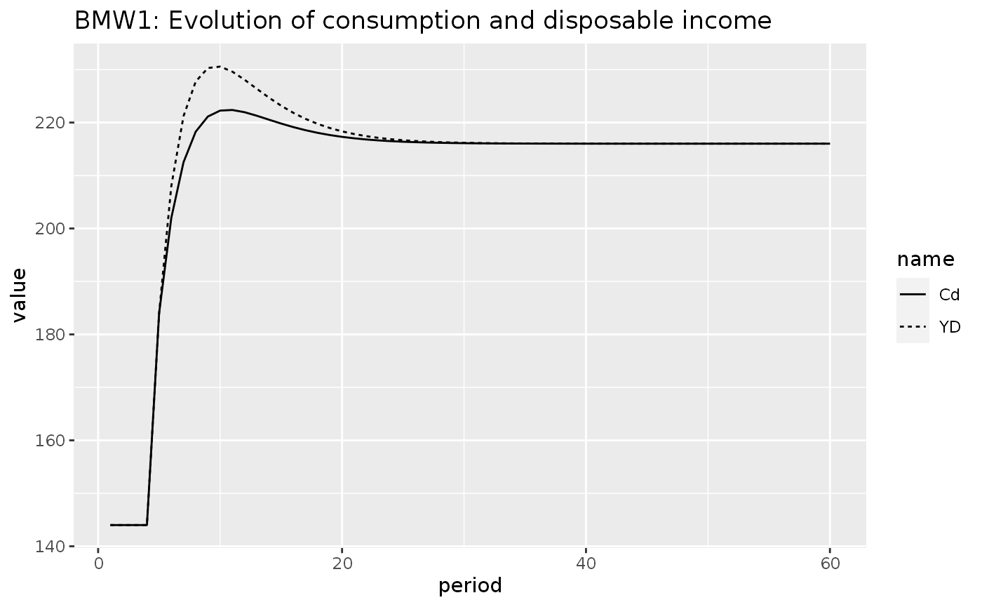
And the investment of firms?
bmw1 %>%
  do_plot(variables = c("Id", "AF"),
          title = "BMW1: Investment of firms")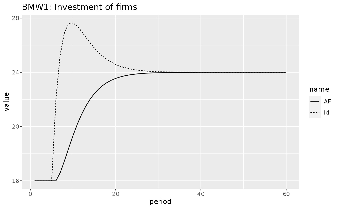
Increase in the propensity to save
shock2 <- sfcr_shock(
  variables = sfcr_set(
    alpha1 ~ 0.7
  ),
  start = 5,
  end = 60
)

bmw2 <- sfcr_scenario(bmw,
                      scenario = shock2,
                      periods = 60)
bmw2 %>%
do_plot(variables = c("Cd", "YD"), title = "BMW2: Decrease in the propensity to save")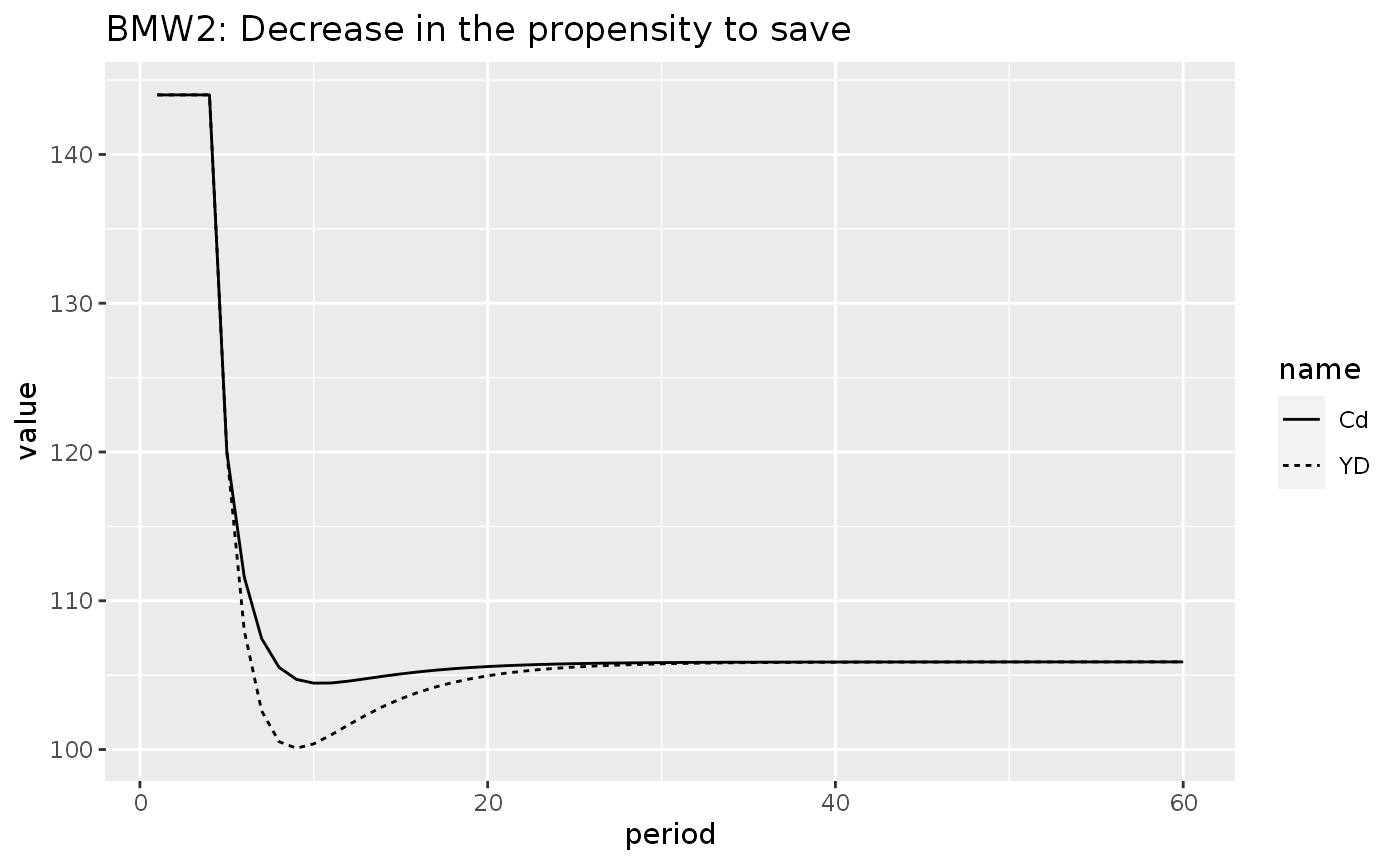 As can be seen, a decrease in the propensity to save in this model leads to a permanent decrease in consumption and on disposable income.
bmw2 %>%
do_plot(variables = c("YK"), title = "BMW2: Decrease in the propensity to save")
#> Warning: Removed 1 row(s) containing missing values (geom_path).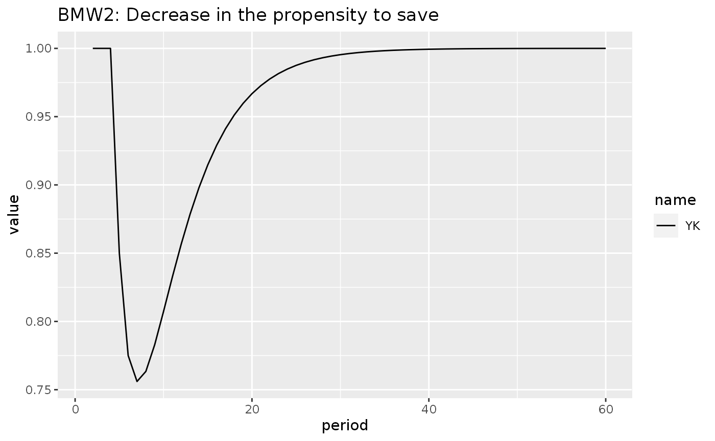 As a note, it is possible to add
 ggplot2 arguments to our helper function:
bmw2 %>%
  do_plot(variables = c("W"), title = "BMW2: Decrease in the propensity to save") +
  labs(subtitle = "Evolution of the real wage")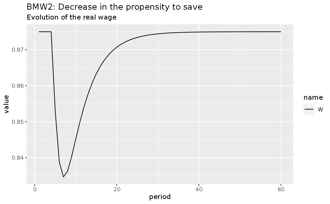
Model BMWK
sfcr_set_index(bmw_eqs) %>%
  dplyr::filter(lhs == "Cd")
#> # A tibble: 1 × 3
#>      id lhs   rhs
#>   <int> <chr> <chr>
#> 1    16 Cd    alpha0 + alpha1 * YD + alpha2 * Mh[-1]

bmwk_eqs <- sfcr_set(
  bmw_eqs,
  Cd ~ alpha0 + alpha1w * WBs + alpha1r * rm[-1] * Mh[-1] + alpha2 * Mh,
  exclude = 16)

sfcr_set_index(bmw_external) %>%
  dplyr::filter(lhs == "alpha1")
#> # A tibble: 1 × 3
#>      id lhs    rhs
#>   <int> <chr>  <chr>
#> 1     3 alpha1 0.75

bmwk_ext <- sfcr_set(
  bmw_external,
  alpha1w ~ 0.8,
  alpha1r ~ 0.15,
  exclude = 3

)
bmwk <- sfcr_baseline(equations = bmwk_eqs,
                 external = bmwk_ext,
                 periods = 100,
                 hidden = c("Ms" = "Mh"),
                 tol = 1e-20,
                 method = "Newton"
                 )
bmwk %>%
  do_plot(variables = 'Y', "BMWK: Steady state")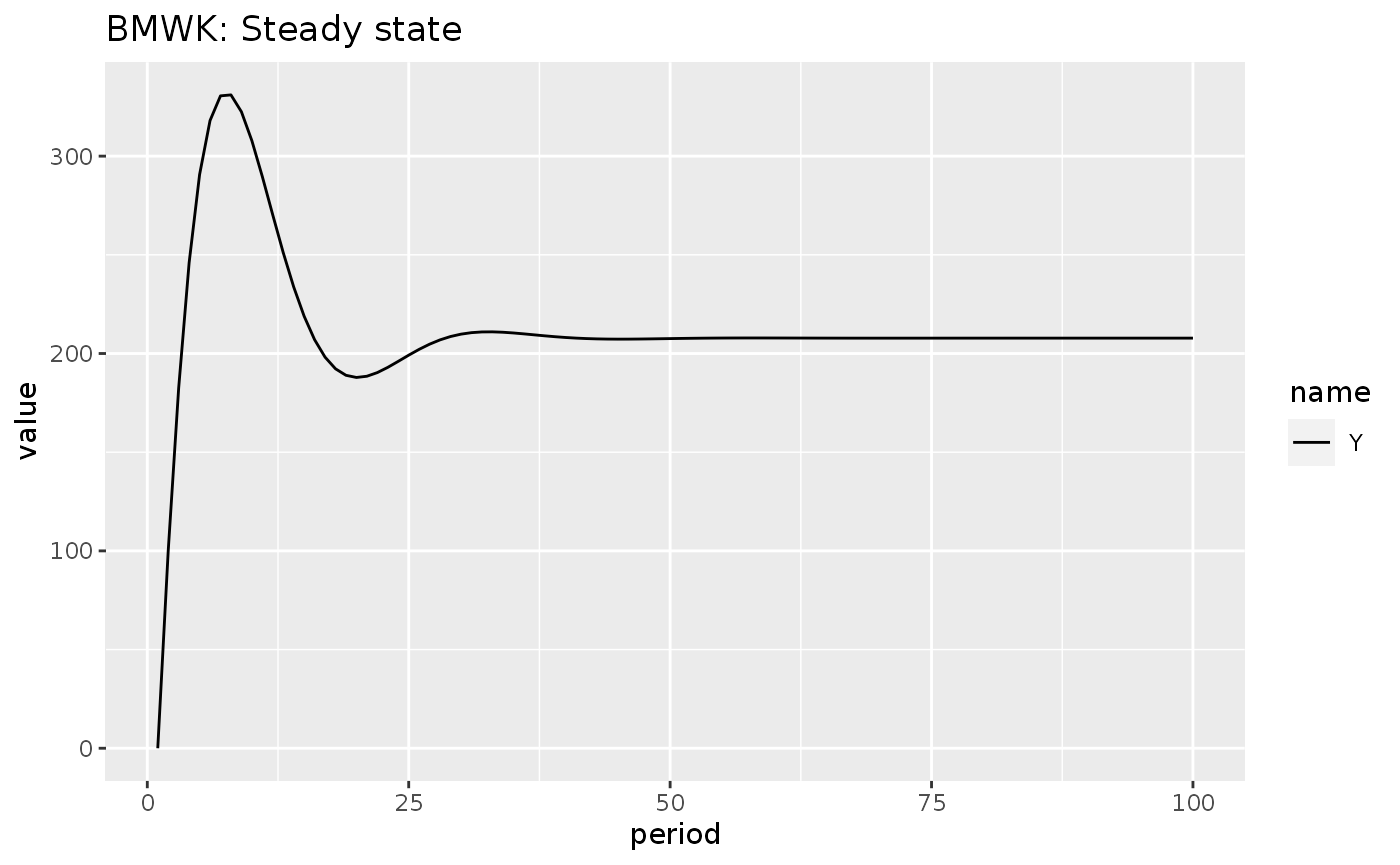
Let’s see the impact of an increase on interest rates in this model:
shock3 <- sfcr_shock(
  variables = sfcr_set(rl ~ 0.035),
  start = 5,
  end = 100
)

bmwk1 <- sfcr_scenario(bmwk, shock3, 100, tol = 1e-10)

bmwk1 %>%
  do_plot("Y", "BMWK1: Increase in the interest rate (rm)") +
  labs(subtitle = "Evolution of Gross Domestic Income (Y)")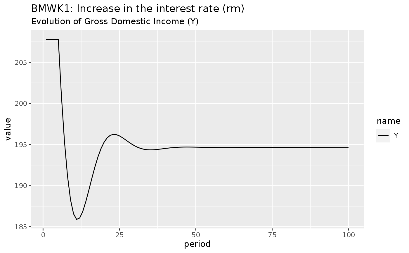
This model has a very interesting characteristic. If we don’t strive for numerical precision with a very small tol argument at the bmw model, the tiny differences in each period lead the model to explosion:
shock3 <- sfcr_shock(
  variables = sfcr_set(rl ~ 0.035),
  start = 5,
  end = 200
)

bmwk1_explode <- sfcr_scenario(bmwk, shock3, 200, tol = 1e-5, method = "Newton")

bmwk1_explode %>%
  do_plot("Y", "BMWK1_EXP: Increase in the interest rate (rm)") +
  labs(subtitle = "Explosion of Gross Domestic Income (Y)")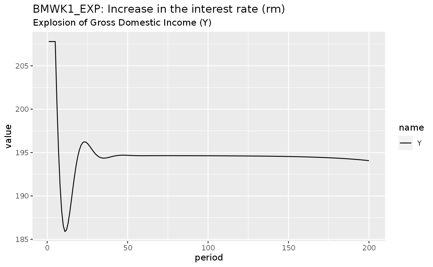
Stability tests
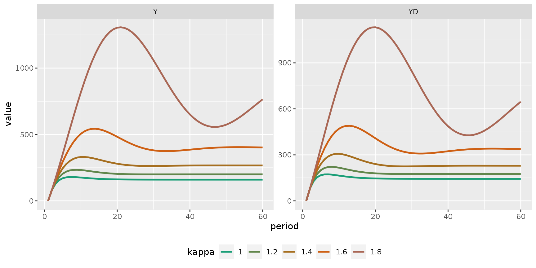
Let’s try to visualize the sensitivity of the model BMW to different parameter values, as discussed in Godley and Lavoie (2007, sec. 7.5.2)
We’ll start by expanding the values of the kappa parameter in the external set:
bmw_xext <- sfcr_expand(bmw_external, kappa, seq(1, 2.6, 0.2))
xbmw <- sfcr_multis(bmw_xext, bmw_eqs, periods = 60, method = "Newton")
We can see that the model start to become very unstable from \(kappa > 1.6\):
getPalette <- grDevices::colorRampPalette(RColorBrewer::brewer.pal(8, "Dark2"))

bind_rows(xbmw[c(1, 2, 3, 4, 5)]) %>%
  mutate(simulation = as_factor(simulation)) %>%
  pivot_longer(cols = -c(period, simulation)) %>%
  filter(name %in% c("Y", "YD", "C")) %>%
  ggplot(aes(x = period, y = value, color = simulation)) +
  geom_line(size = 1, alpha = 1) +
  theme(legend.position = "bottom") +
  scale_color_manual("kappa",
     values = getPalette(20),
     labels = as.character(seq(1, 2.6, 0.2))) +
  facet_wrap(~ name, scales = 'free_y')